Using Facebook’s Prophet, an open-source, time series forecasting procedure to predict SPY (SPDR S&P 500 ETF Trust) closing prices.
tl;dr
Goal
To apply Facebook's Prophet forecasting procedure to historical SPY (SPDR S&P 500 ETF Trust) market data to gather future pricing predictions.
A few notes
- I'm by no means a data scientist, so this is more of an exploratory analysis than an accurate one
- For sake of brevity, I won't be using a training/test split or measuring the error of the model, I will just train the model on the entire dataset and then make a prediction
Process overview
- Downloading the data - exporting the data from Yahoo Finance as a CSV
- Exploring the data - loading and exploring the data using Pandas
- Fitting the model - reading in the data and applying a basic fit of the Prophet model to the data
- Visualizing the forecast - visualizing the forecasted pricing data
Python dependencies
import pandas as pd
from prophet import Prophet
Important This article is not investment advice, please conduct your own due diligence. This is merely a simple analysis.
Before we jump in, let's give a little background on SPY and on Facebook's Prophet.
The SPDR S&P 500 ETF Trust (SPY) is an ETF (Exchange Traded Fund) that tracks the performance of the S&P 500 index. SPY is also the largest ETF in the world, and is popular compared to other ETFs that track the S&P 500 because of the high volume, or the number of shares that trade on a given day (we'll be able to see the volume per day in the CSV we export from Yahoo Finance).
For more information on ETFs, Investopedia gives a good overview.
Facebook Prophet is an open source, automated forecasting procedure for time series data. I'm not going to dive too much into the mathematics or implementation details of Prophet, but if you are more interested, you can read the research paper. Prophet makes it easy to handle outliers, adjust to different time intervals, deal with holidays, and leaves the ability to easily tune the forecasting model.
Now that we have a general idea of what we're trying to predict and the tool we'll use to forecast, let's dive into the actual data.
Downloading the data
Thanks to Yahoo Finance, we can download historical pricing data for free. You can click here to view the SPY historical pricing data.
Click on the Historical Data tab, and then we can adjust our Time Period to the Max as seen below (back to January 1993).
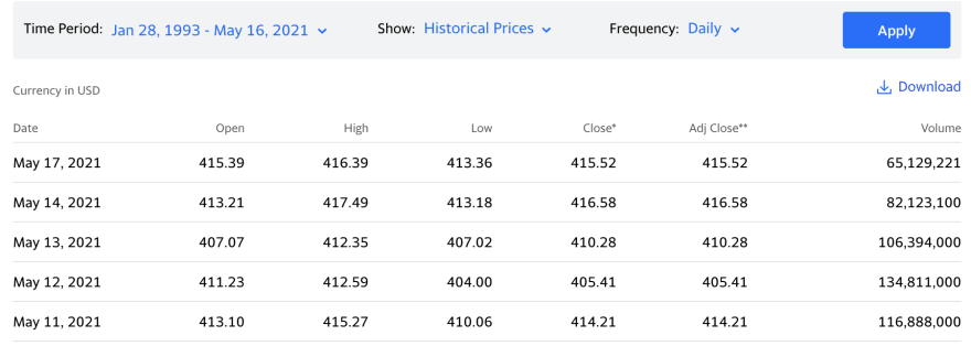
Now we can click download to get our CSV and start diving into the data.
Exploring the data
Let's fire up Pandas and load our data into a DataFrame to see what general insights we can extract.
df = pd.read_csv('SPY.csv')

# Columns and row count
df.info()
"""
<class 'pandas.core.frame.DataFrame'>
RangeIndex: 7125 entries, 0 to 7124
Data columns (total 7 columns):
 #   Column     Non-Null Count  Dtype
---  ------     --------------  -----
 0   Date       7125 non-null   object
 1   Open       7125 non-null   float64
 2   High       7125 non-null   float64
 3   Low        7125 non-null   float64
 4   Close      7125 non-null   float64
 5   Adj Close  7125 non-null   float64
 6   Volume     7125 non-null   int64
dtypes: float64(5), int64(1), object(1)
memory usage: 389.8+ KB
"""

# Preview of the data
df.head()
"""
         Date      Open      High       Low     Close  Adj Close   Volume
0  1993-01-29  43.96875  43.96875  43.75000  43.93750  25.884184  1003200
1  1993-02-01  43.96875  44.25000  43.96875  44.25000  26.068277   480500
2  1993-02-02  44.21875  44.37500  44.12500  44.34375  26.123499   201300
3  1993-02-03  44.40625  44.84375  44.37500  44.81250  26.399649   529400
4  1993-02-04  44.96875  45.09375  44.46875  45.00000  26.510111   531500
"""

# General statistics
df.describe().loc[['mean', 'min', 'max']]
"""
            Open        High         Low       Close   Adj Close        Volume
mean  146.896395  147.766581  145.928716  146.896373  121.611954  8.453727e+07
min    43.343750   43.531250   42.812500   43.406250   25.571209  5.200000e+03
max   422.500000  422.820007  419.160004  422.119995  422.119995  8.710263e+08
"""

# Day to day percent changes of Highs
df[['Date', 'High']].set_index('Date').pct_change().reset_index()
"""
            Date      High
0     1993-01-29       NaN
1     1993-02-01  0.006397
2     1993-02-02  0.002825
3     1993-02-03  0.010563
4     1993-02-04  0.005575
         ...       ...
7120  2021-05-10 -0.000189
7121  2021-05-11 -0.017670
7122  2021-05-12 -0.006454
7123  2021-05-13 -0.000582
7124  2021-05-14  0.012465

[7125 rows x 2 columns]
"""
Now that we know a bit more about our data in general, we can create a model using Prophet.
Fitting the model
Since we're not concerned in this post about making our model the best it can be, we can train our model on the entire dataset.
This typically isn't a good practice. When trying to make an accurate prediction, you should use training and test subsets of the data and calculate errors within your model and use those results to tune hyperparameters.
Nevertheless, let's continue.
# The prophet model fits to a DataFrame with a date column (ds)
# and a value to predict (y)
df_predict = df[['Date', 'Close']]
df_predict.columns = ['ds', 'y']

# We can find all of the missing days within our dataset
# and mark those as "holidays"
date_series = pd.to_datetime(df['Date'])
df_missing_dates = pd\
    .date_range(start=date_series.min(), end=date_series.max())\
    .difference(date_series)\
    .to_frame()\
    .reset_index()
df_missing_dates.columns = ['holiday', 'ds']
df_missing_dates['holiday'] = 'Stock Market Closed'

# Fitting our model is incredibly simple and can be done in the
# most basic sense in just two lines of code
m = Prophet(daily_seasonality=True, holidays=df_missing_dates)
m.fit(df_predict)
Just like that, we have built our model for a forecast. All we have left to do is generate dates to predict values for, and run the actual prediction.
Visualizing the forecast
Now let's forecast with our model and visualize the results.
# Create a DataFrame with past and future dates (only weekdays)
future = m.make_future_dataframe(periods=365)
future = future[pd.to_datetime(future['ds']).dt.weekday < 5]

# Now we can forecast and visualize in just two more lines of code
forecast = m.predict(future)
m.plot(forecast, xlabel='Date', ylabel='Daily Closing Price')

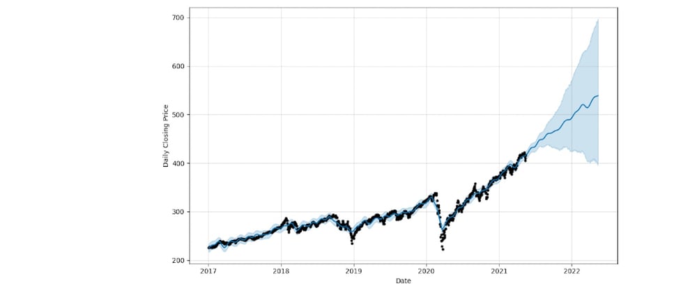
A few things to notice
- The black dots are the training data points
- The blue outline is the confidence interval
- The line within the confidence interval is the actual forecast
Based on our results, we can see the forecast is fairly linear and the confidence interval is relatively narrow (due to the volume of date). The behavior of the stock market since Covid-19 started back around February 2020 has be a little unorthodox, so let's narrow our model to be trained back to data starting in 2017 to see if there is an effect.
# Narrow down to start at 2017
df_recent_predict = df_predict.iloc[date_series[date_series.dt.year > 2016].index]
date_series = pd.to_datetime(df_recent_predict['ds'])
df_recent_missing_dates =  pd\
    .date_range(start=date_series.min(), end=date_series.max())\
    .difference(date_series)\
    .to_frame()\
    .reset_index()
df_recent_missing_dates.columns = ['holiday', 'ds']
df_recent_missing_dates['holiday'] = 'Stock Market Closed'

# Create and fit our new model
m = Prophet(daily_seasonality=True, holidays=df_recent_missing_dates)
m.fit(df_recent_predict)

# Recreate our future predictions
future = m.make_future_dataframe(periods=365)
future = future[pd.to_datetime(future['ds']).dt.weekday < 5]

# Forecast and visualize
forecast = m.predict(future)
m.plot(forecast, xlabel='Date', ylabel='Daily Closing Price')

Now we can see a much wider confidence interval and a bit more of a bumpy forecast line; however, this looks much more realistic in terms of stock market prediction.
Conclusion
All in all, Facebook's Prophet is a very fast, impressive, and strongly abstracted library. The entire script, including reading in the data, training and forecasting two models, and plotting both of the forecasts took right around 25 seconds.
I would love to see this tool in the hands of an actual data scientist to see the accuracy of the models they'd be able to create using Prophet.


Top comments (0)