
Last week we saw some ways to evaluate a machine learning model but they were only for classification problems. Let's see another way to evaluate one and then focus on regression model evaluations.
Table of contents:
Confusion matrix
The confusion matrix is a way to compare what the machine predicted with what it was supposed to predict, it gets this name because lets us know where the model is getting confused and predict a label instead of another. Using the same estimator of the last week we can already import what we need:
from sklearn.model_selection import train_test_split
from sklearn.svm import SVC

X = iris_df.drop('target', axis = 1)
y = iris_df['target']

X_train, X_test, y_train, y_test = train_test_split(X, y, test_size = .15)

clf = SVC()
clf.fit(X_train, y_train)

y_preds = clf.predict(X_test)
now we can import the function to do the confusion matrix:
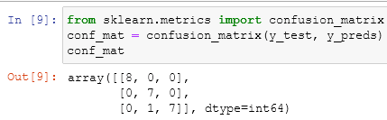
But what does this mean? It is based on the false positive rates (fpr) and true positive rates (tpr), which we saw in the last post. Every cell of the matrix indicates if the model predicted correctly or not the class. We can have a quick overview with the pandas function crosstab:

Knowing that 0, 1, and 2 are our labels Setosa, Versicolor, and Virginica, we can see where the model predicted a right label and where a wrong one.
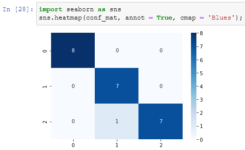
Having saved the result of the confusion_matrix function into conf_mat we can even import the seaborn library to plot it in an utterly fashion way:
Regression model evaluators
Till now we saw just how to evaluate a classification model and how to use a binary classification evaluator for multi-class classification. Evaluating a regression model is much simpler than what we already did despite being vital to machine learning in general
Coefficient of determination
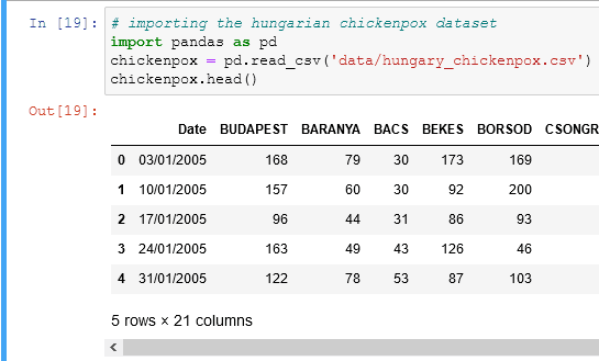
the coefficient of determination or R^2 (R-squared) is the score method that we saw from the begin of the serie, but let's understand how does it work. Let's begin importing a regression dataset:
 you can find the data here
looking at the data we know that we have all the cases of chickenpox in Hungary divided by county areas. We want to predict the total cases based on how many cases were in every county. We'll create column with the total cases for every day, to do so we need a single line of code:
chickenpox['total'] = chickenpox.sum(axis = 1)
this will create an additional column with the sum of all the cases in every row:

Now we can fit and train our model:

The result is the same which we already saw thousands of times: a number between 0.0 and 1.0 which correspond to a percentage. The coefficient of determination compares every prediction with the test label. We can use the dedicated function from the library to calculate it:

because the R-squared scores compare two multi-dimensional arrays, if we compare the test with itself we'll get a score of 100%: 1.0

The Mean Absolute Error (MAE)
the mean absolute error score calculates the absolute difference between every actual value and every predicted one:

Absolute means that every number is positive, so a complete way to do the dataframe would be:

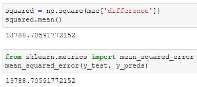
To complete this evaluation we have to just calculate the mean of the difference column. Let's compare our calcs with the dedicated function:
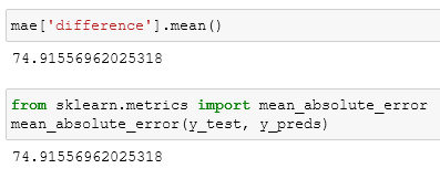
And from what we can see we did everything right.
The MAE tells us the range of the error of our model, through this evaluation, we now know that the errors of our model range between 74 and -74.
The Mean Squared Error (MSE)
The mean squared error is identical to the MAE but every value of the difference column is squared:
When to use them?
- R-squared is used for accuracy but doesn't tell you where the model is doing wrong.
- MAE gives a good indication of how wrong your model is
- MSE amplifies larger differences than MAE
In this case, if 200 cases are twice as bad as 100 cases we could use the MAE, but if a disease has a very high rate of transmission then 200 cases would be more than twice as bad as 100 and we should pay more attention to the MSE.
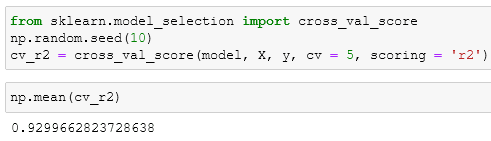
Using the scoring parameter
We can have the same results using the cross-evaluation function and changing the scoring parameter:
for the full list, you can go here
Last thoughts
We saw all the most important ways to evaluate our machine learning model avoiding using mindlessly the metrics functions without knowing what they do. If you have any doubt feel free to leave a comment.


Top comments (0)