
In this week we'll see the final part of all the functions that we may need to use numpy in our machine learning project.
Let's dive in!
table of contents:
- Viewing the operation performance
- Reshaping and transposing
- Matrix multiplication
- Comparison operators
- Sorting arrays
- Finding the maximum value of an array
- Final thoughts
Viewing the operation performance
In python, using numpy, as well as other languages, we'll have a lot of ways to do the same thing; In python, we have the sum function and with numpy we have to np.sum function too.
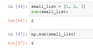
As you can see both returns the same result, leaving a question:
When is a function better than the other?
Num is the official python function to sum python lists, while the np.sum function is the official function to sum numpy arrays, which are the same thing conceptually, but not when the machine has to perform the calculation.
The best way to act is to use python function for python data types (in this case lists) and numpy functions for numpy data types (numpy arrays and types).
But an even more important difference besides the performance of these two functions. With some special numpy functions (characterized by the % at the beginning) we can display the time that the machine took to perform the operations, in this case, we'll use %timeit.
We'll first create a big array:

for then using the timeit function:

Using the google converter we can see that the python sum took 2.28 milliseconds, while the numpy sum took 13 microseconds, being more than 500 times faster.
Reshaping and transposing
As we already stated, one of the most important things to be sure in our carrier in machine learning is that data fit other data, let's see it with an example.
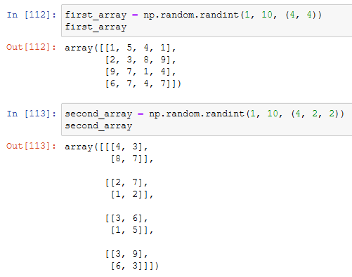
Let's begin with creating two different arrays with different shapes:
Not let's try to multiply them together:

The error says that two arrays with different shapes cannot be broadcasted together. If we go on the numpy documentation we can see that the general rule for broadcasting says:
When operating on two arrays, NumPy compares their shapes element-wise. It starts with the trailing (i.e. rightmost) dimensions and works its way left. Two dimensions are compatible when
- they are equal, or
- one of them is 1
That means that we have to reshape our array, and we can do it with the numpy reshape function:

Now that the first array corresponds to the main rule of broadcasting we can multiply the two arrays together:

Note that the reshape function follows precises rules and that this is just an example, an array cannot be always reshaped into something different.
Now that we have seen the reshape function let's see the transpose one.
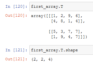
As we can the transpose function, which we call with a "T", simply swap the axis of an array between them.
Both reshape and transpose are very useful function that will come in very handy when we'll have to do multiplicate two - or more - matrices
Matrix multiplication
Multiplying a matrix by a single number or a one-dimensional array is fairly easy, but multiplying a matrix by another matrix is something that will be a bit tough to understand but very important.
There are two ways to multiplicate array for each other:
Element wise
An element-wise multiplication is very easy and can be done only between arrays of the same size:

and we can do it with the numpy function:

Dot product
Note: in the following examples there is an error in the matrix: it has the 5 instead of 4 and viceversa.
The other one is specific for matrices and if you don't understand it on the first try, don't worry, is simple if you understand what's going on.

But this, at first glance, can still be confusing. Let's see it with some colors:

As you can see, we took the first array with the matrix with '1', '2', and '3' and multiplied it for 'A', 'B' and 'C'. This is commonly called the waterfall method. You can understand why viewing the animation here.
As a general rule, to multiply two matrices together they need to be aligned. Let's see what happens if we try to use the dot product on the matrices that have multiplied element-wise, using the dot function:

As you can see they are not aligned. Two matrices are aligned when the the row o of the first is the same as the column of the other, or: m x n * n x p. This way we know that the result will be a matrix that is m x p:
m x n * n x p = m x p
that in our case could be:
3 x 2 * 2 * 3 = 3 * 3
that means that two matrices can be multiplied. In our case we have to transpose the axis:

In our case we got as result a 2 x 2 matrix, as we already saw:
2 x 3 * 3 x 2 = 2 x 2
Exactly as we expected. If we would have transposed the first matrix the result would have been a 3 x 3 matrix.
To see the dot product from a mathematical point of view you can read here.
Comparison operators
Between arrays and matrices we can even do comparisons. The result will be another boolean array. Let's see an example:

We can use all the logical operator that we used in our programming carrier, but it's important to know that the comparison follows the same rules of broadcasting:

Sorting arrays
Numpy offers various functions for finding an element and for sorting an array. The most common way is sort, that sort when applied on a matrix every row of it.

Finding the minimum value of an array
To find the minimum value of an array numpy offers the argmin function, that returns the index of the lowest value:

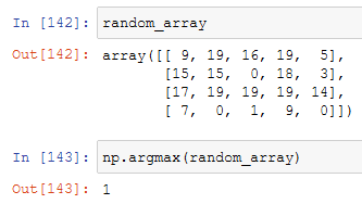
Finding the maximum value of an array
If to find the minimum we use argmin, to find the maximum we find argmax:
more on argmin and argmax
Both the function let us enter the axis of the array so that we can find the maximum or the minimum not of all the array but of all the columns or rows:
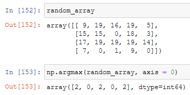
With the axis set on 0, it will find the maximum of all the columns, if set on 1 of all the rows.
Final thoughts
This and last week we saw the numpy library to manipulate arrays and matrices, the datasets that we'll have in machine learning. Next week we'll see matplotlib to visualize our data, for then focusing on something more practical. If you have any doubt feel free to leave a comment.


Oldest comments (0)