How I am learning machine learning - week 5: python and matplotlib (part one)

We know about pandas and numpy and after matplotlib, we'll know the core of machine learning; the prior knowledge needed to make actually a good project and how these three library matches so much together, so let's dive in!

Table of contents:

• Importing matplotlib
• 3 methods to make a plot
• Figure vs. plot
• Making a scatter plot
• Making a bar plot
• Making a histogram plot
• Making a figure with plots in it
  • The-second way to make a figure
• Final thoughts

Importing matplotlib

To get the maximum from matplotlib we can't just import it, we have to add a special line first:

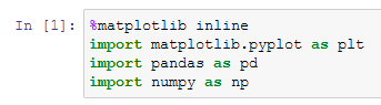
%matplotlib inline will display the plot, or the figure(more later on), into our notebook, without we would have just a series of fancy numbers as output.

The principal function in matplotlib is plot, and is used to display a simple x and y graph:

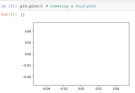
to don't see the square brackets, or any other additional line, we put a ';' at the end:

but we are going to do more than create void graphs, so let's see a practical example of a graph:

3 methods to make a plot

In matplotlib there are various ways to make a plot and everyone has a specific purpose, but the recommended method is the most simple:

plt.plot(x, y)

that we already saw. The second method makes you write:

ax = plt.subplot()
ax.plot(x, y)

so that you can display multiple figures in the same plot. The third method will be similar to:

figure = plt.figure()
axes = fig.add_axes ([5, 10, 15, 20])
ax.plot (x, y)
plt.show()

All of this will lead to the same results for now. The first and the second method will go together later on to create powerful and highly customizable plots. If you want to read more about them you can see [this StackOverflow question].
(https://stackoverflow.com/questions/37970424/what-is-the-difference-between-drawing-plots-using-plot-axes-or-figure-in-matpl)

Figure vs. plot

There is an important distinction to know in matplotlib: the difference between a plot and a figure.
A plot is simply the graph that displays the data, while the figure is the container of the plot. This way one can have more plots in the same figure while customizing the singular plot.
This is all summarized by the image made by Daniel Bourke for his course on zero to mastery.

source

Here we can introduce the object-oriented method to actually create plots and subplots.
The most common line that you'll see online will be similar to:

fig, ax = plt.subplots()

Here we are creating the figure and the axis object. Axis is the canvas where you can put and customize all your data and every axis can belong to only one figure.
We call the subplots function on two objects because it returns a tuple
may contain one or more plots of the figure. Now we can call the plot function on the ax object:

ax.plot(x, y)

And this will display the same graph that we saw earlier, the difference is that now it is customizable:

ax.set(title = "example plot", xlabel = "x_axis", ylabel = "y_axis")

And with these commands we have created our figure with a plot inside of it; but an important function, that comes at the end of a project, is savefig:

fig.savefig("images/example-figure.png")

Usually, this happens through various steps, but now you'll see it in just one bite so that everything can be clear:

Making a scatter plot

Now that we know enough of the matplotlib foundamentals we can begin making some real figures. The first we'll see is the scatter plot. We'll use the linspace function to create the array. It returns evenly spaced numbers over a specified interval. 50 by default:

Note that you can see just the first 10 using [:10] or whatever numbers you want.

Making another plot we have to initialize the figure and plot again to avoid errors:

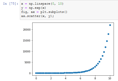
Instead of putting into y the exponential of x we could have typed ax.scatter(x, np.exp(x)) but I preferred to do this way to be more clear.

Making a bar plot

The making of a bar plot in matplotlib is a great way to know that we can make a plot out of a dictionary too:

Making a histogram plot

The best way to explain a histogram is through the randn function, which generates a normal distribution of random numbers. The following example is similar to one in the documentation but more direct and simpler:

Making a figure with plots in it

We said earlier that a figure is a container for plots and now we'll see how to do it.

For making a figure there are two options. The one that you'll see is what I find more readable and is usually a good practice in programming.

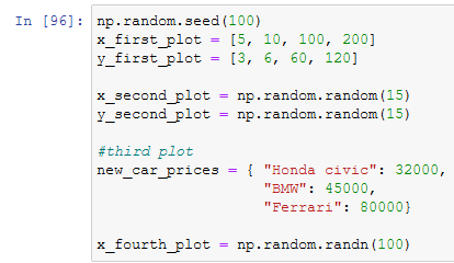
First of all, we define all the values of our plots, so that everything can be more clear:

np.random.seed(100)
x_first_plot = [5, 10, 100, 200]
y_first_plot = [3, 6, 60, 120]

x_second_plot = np.random.random(15)
y_second_plot = np.random.random(15)

#third plot
new_car_prices = { "Honda civic": 32000,
               "BMW": 45000,
               "Ferrari": 80000}

x_fourth_plot = np.random.randn(100)

After having declared all our data we'll press shift + enter and begin the making of the figure. At the first line that we'll see:

figure, ((first_plot, second_plot), (third_plot, fourth_plot)) = plt.subplots(nrows = 2, ncols = 2, figsize = (12, 6))

Here we are declaring the figure and the axis. Every axis is a single plot. The subplots figure returns a tuple with two values: the figure and the plots, so to make the figure we have to pass into the function determined values. In this case, we want a figure with 2 rows ("nrows = 2"), two columns ("ncols = 2"), and a figure that has a size of 8 as width and 4 as height ("figsize = (12, 6)"). The values of the size of the figure are arbitrary and will determine the size of the image that will be the figure.

Now that we have declared all of our axis we can customize everyone of them:

first_plot.plot(x_first_plot, y_first_plot);
second_plot.scatter(x_second_plot, y_second_plot);
third_plot.set(title= "car seller prices", ylabel="price ($)");
third_plot.bar(new_car_prices.keys(), new_car_prices.values());
fourth_plot.hist(x_fourth_plot);

Now that we have done everything we can see the final results:

In the real case we would have a bigger figure, here is small to put it all in the screenshot.

And after all of this, we would make an image of this so that the final product may be similar to:

The second way to make a figure

The second way to make a figure, that is less used but still important to know, is to make just an array/matrix plot and use his indexes to refers to the various plot. In practice it looks like:

figure, plot = plt.subplots(nrows = 2, 
                            ncols = 2,
                            figsize = (15, 10))

plot[0, 0].plot(x_first_plot, y_first_plot);
plot[0, 1].scatter(x_second_plot, y_second_plot);
plot[1, 0].set(title= "car seller prices", ylabel="price ($)");
plot[1, 0].bar(new_car_prices.keys(), new_car_prices.values());
plot[1, 1].hist(x_fourth_plot);

This will produce the same results that we already saw.

Final thoughts

Today we saw the foundamentals of matplotlib. The following week we'll see how all of this goes together with pandas and numpy.
If you have any doubt, feel free to leave a comment.