Astronomical computing – Ep 6 - Solving Kepler's equation in Ruby

One of the main goals of this series is to understand the math behind astronomical events calculations, and translate them into simple and maintainable code.

In order to forecast where a planet will be visible in the night sky at a given moment we need to rely on topics that we haven’t yet covered such as orbital elements.

Unlike far away stars which can be considered motionless^[1], planets change position on the celestial sphere from one night to the other. Even the Sun, from our point of view, seems to be slowly moving alongside the zodiac belt throughout the year. Our first step towards finding out where a planet will be visible in the sky is to calculate its equatorial coordinates.

Kepler's second law states that the orbital speed of an object varies throughout its orbit. With an elliptic orbit and a changing speed, calculating the planet's location on its orbit for a known date is not a linear process.

We won't cover the calculations needed to compute the coordinates of a planet in this article. We will make sure to cover those in a later installment though. Still, this is an essential step to understand a planet’s motion on its orbit.

Some definitions

Almost all of the following content can be traced to one single source: Celestial Calculations, A Gentle Introduction to Computational Astronomy, by J. L. Lawrence, editions MIT Press.

This is not the first time I mention this book as it is one of my main sources for this series, and I cannot be more grateful of the incredible work of communication and explanation the author has produced to make all these phenomenons accessible.

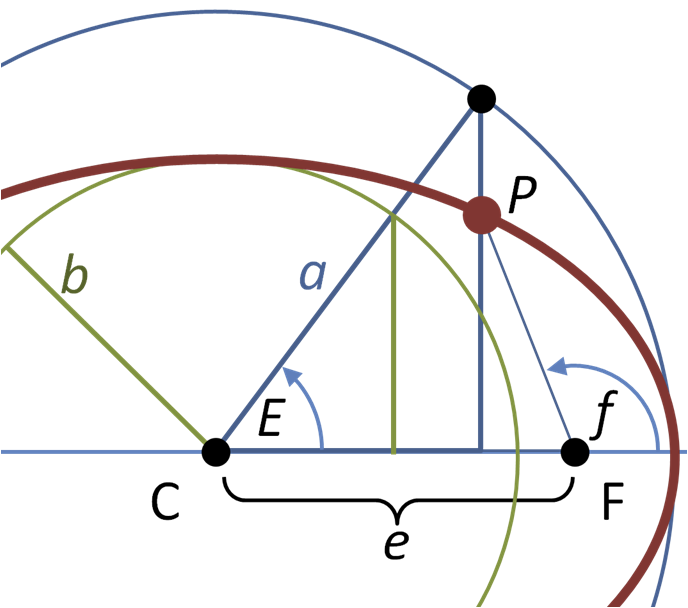
Section of ellipse showing eccentric and true anomaly^[2]

The illustration above will be useful to understand the different definitions:

• The red ellipse is the true anomaly
• The blue circle is the mean anomaly
• F is the main focus
• C is the geometrical center of both the red and blue circles
• f is the true anomaly
• E is the eccentric anomaly

True anomaly

We can consider it as being the angle between the body's current position and its periapsis, as seen from the main focus of the ellipse. I can imagine how this definition is not helping, so let's go a bit further.

The main focus of the ellipse is basically the point around which the body rotates. When talking about planets of the Solar System, this point can be considered as the Sun^[3].

The periapsis is the nearest point on the orbit to the main focus. For planets, it's called perihelion and is the point where it's the closest to the Sun.

In other words, the true anomaly is the angular distance between the current position and a fixed point, as seen from the Sun.

Mean anomaly

As a planet's orbit is an ellipse and its speed changes constantly depending on how close it is from the Sun, it's pretty difficult to calculate the true anomaly.

To tackle this non trivial task, scholars imagined a fictive orbit, circular, on which the body would move with a constant speed, called the mean orbit. The real orbit would share its geometrical center and its periapsis with the mean orbit's center, which means the body would have the same orbital period on both orbits.

The mean orbit is the angle, from the fictive circle's center, between the body's current position and the periapsis.

The mean orbit is considerably easier to use. A body's mean position on its mean orbit with an orbital period of n sidereal days, after t days from a starting point (the periapsis), can be described this way:

mean_anomaly = 360 / n * t

Eccentric anomaly

The eccentric anomaly is another angular parameter that helps defining the position of a body on its orbit.

It is the projection of the body's current position on the mean orbit, parallel to the line that goes through the mean orbit's center and the periapsis.
Technically we don't use the mean orbit but a circle called the auxiliary circle, but they're the same circle.

Knowing the orbital eccentricity, and the eccentric anomaly, the true anomaly can be defined as:

true_anomaly = arc_tangent(
  square_root(
    (1 + orbital_eccentricity) / (1 - orbital_eccentricity)
  ) * tangent(eccentric_anomaly / 2)
) * 2

Okay, yes, this is getting weirder and weirder but please bear with me, we're getting closer.

Kepler's equation

Kepler discovered that the eccentric and the mean anomalies are related by the following equation:

mean_anomaly = eccentric_anomaly -
  orbital_eccentricity * sine(eccentric_anomaly)

where the mean and eccentric anomalies are expressed in radians.

Knowing this relation, all we have to do is to use the orbit’s orbital eccentricity along with the mean and eccentric anomalies to finally calculate the true anomaly. The calculation for the orbital eccentricity of an orbit is not covered in this article, so we can consider that we already know its value.

Iterations

Unfortunately, Kepler's equation is a transcendental equation, there is no known closed-form solution for it. To compute the eccentric anomaly, we must resolve the equation iteratively and get the most accurate approximation as possible.

If two consecutive iterations have a difference inferior to a pre-defined accuracy parameter, then we can use the last iteration' solution as the most accurate approximation.

Instead of resolving the equation defined above, we will resolve another one, defined as the Newton/Raphson method, which is known to be more performant and more accurate.

Iteratively, we will resolve the following equation:

eccentric_anomaly(i) = eccentric_anomaly(i-1) - (
  (
    eccentric_anomaly(i-1) -
      orbital_eccentricity * sin(eccentric_anomaly(i-1)) -
      mean_anomaly
  ) / (
    1 -
    orbital_eccentricity * cosine(eccentric_anomaly(i-1))
  )
)

where i represents the following the current iteration.

For the first iteration, where i is 0, we will have the following fixed solution:

• mean_anomaly if the orbital eccentricity is 0.75 or less,
• π if the orbital eccentricity is more than 0.75.

Finally, we will also introduce a maximum number of iterations, as some configuration may lead to values that never converge, and to prevent from a too small accuracy parameter.

Implementation in Ruby

Finally the part that actually matches the article's title.

The implementation is actually quite simple and uses recursion. This is one solution, other interesting implementations might be available out there.

def kepler_equation_newton_raphson_iteration_scheme(
  mean_anomaly_in_radians,
  orbital_eccentricity,
  precision,
  maximum_iteration_count,
  current_iteration = 0,
  solution_on_previous_interation = nil
)
  solution = if current_iteration == 0
    if orbital_eccentricity <= 0.75
      mean_anomaly_in_radians
    else
      Math::PI
    end
  else
    solution_on_previous_interation - (
      (
        solution_on_previous_interation -
        orbital_eccentricity *
        Math.sin(solution_on_previous_interation) -
        mean_anomaly_in_radians
      ) / (
        1 -
        orbital_eccentricity *
        Math.cos(solution_on_previous_interation)
      )
    )
  end

  if solution_on_previous_interation
    delta = solution - solution_on_previous_interation
    puts "E#{current_iteration} ≈ #{solution}, " \
    "Δ = #{delta.ceil(6).abs}"
  else
    puts "E#{current_iteration} ≈ #{solution}"
  end

  if current_iteration >= maximum_iteration_count ||
      (
        solution_on_previous_interation &&
        delta.abs <= precision
      )
    return solution
  end

  kepler_equation_newton_raphson_iteration_scheme(
    mean_anomaly_in_radians,
    orbital_eccentricity,
    precision,
    maximum_iteration_count,
    current_iteration + 1,
    solution
  )
end

Nothing fancy here, we compute the current iteration' solution from the previous iteration' solution, unless it is the first iteration. Recursion helps computing each iteration and passing the previous iteration' solution.
As long as we have two solutions to compare, we check if their difference is significant, and if we have some iterations left before having to stop manually.
I also added some logs to have a better view of what's happening.

To illustrate this implementation, let's solve Kepler's equation with the Newton/Raphson method for an orbital eccentricity of 0.5 and a mean anomaly of 24.742896°.

First we have to convert the mean anomaly from degrees to radians:

radians = degrees * π / 180
        = 0.431845

Then, we set the accuracy parameter to 0.000002 radians, which is around 0.4 arc seconds.
We set the maximum number of iterations to 10.

Finally, we convert the solution from radians to degrees.

kepler_equation_newton_raphson_iteration_scheme(
  0.431845,
  0.5,
  2e-06,
  10
) * 180.0 / Math::PI

# E0 ≈ 0.431845
# E1 ≈ 0.8151984038210852, Δ = 0.383354
# E2 ≈ 0.7856420972684516, Δ = 0.029556
# E3 ≈ 0.7853985310762203, Δ = 0.000243
# E4 ≈ 0.7853985148507631, Δ = 0.0

# => 45.00002013679163

The expected answer is 45°, which differs of only 0.073" from the solution we computed.

Conclusion

The true anomaly is one step towards our ability to compute where a planet is supposed to appear on the celestial sphere for a given time from a given place on Earth. We are one step closer to this goal and we already have the Ruby implementation ready.

This also helped us understand why we need this value and in what way it is not straightforward to compute it.

---

• ^[1] This is absolutely false as everything in space moves, all the time, depending on the referential. Far away stars also rotate around the galaxy's center. The only difference with planets is that their motion appear extremely slow from our point of view, so slow that we often looks like they are fixed compared with short periods of time such as a Human life.
• ^[2] Source: Wikimedia Commons. Author: Brews ohare.
• ^[3] In reality the planets orbit around the Solar System barycenter, which moves through time due to the different positions of planets. It is always located between the Sun's center and its corona, so we usually consider the Sun itself as the barycenter.