If you want to perform a multi-criteria lookup and transpose results into a table, you can use an array formula based on the INDEX and MATCH functions. Let’s see them below!! Get an official version of ** MS Excel** from the following link: https://www.microsoft.com/en-in/microsoft-365/excel

Generic Formula:
- Use the below formula to get the transpose results.
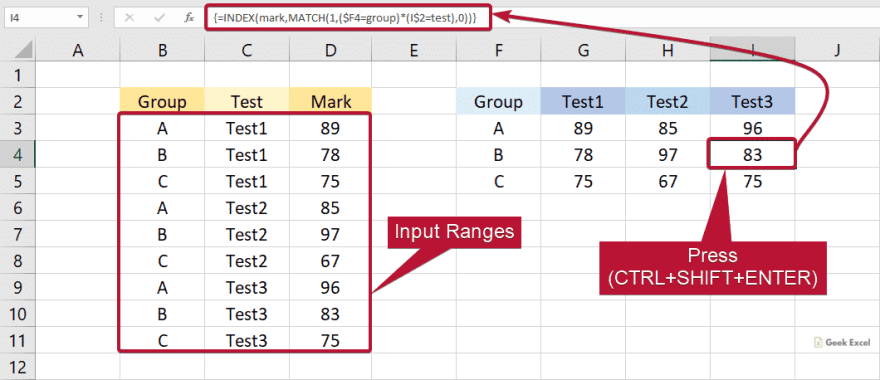
=INDEX(range1,MATCH(1,($A1=range2)*(B$1=range3),0))
Syntax Explanations:
- INDEX – In Excel, the INDEX function will help to return the value at a given position in a range or array.
- MATCH – The MATCH functionin Excel is used to locate the position of a lookup value in a row, column, or table.
- Absolute Reference ($) – The absolute reference is an actual fixed location in a worksheet.
- Comma symbol (,) – It is a separator that helps to separate a list of values.
- Parenthesis () – The main purpose of this symbol is to group the elements.
- Range – It represents the input data given in the worksheet.
- A1, B1 – It represents the criteria.
- Multiplication (*) – In this symbol will multiply any two values or numbers.
Practical Example:
Please do as follows to look up the table with transpose results. Refer to the below example image.
- First, we will enter the input values in Column B , Column C , Column D.

- Now, we are going to sort out the table as shown below and look up the values based on the given criteria.

- Enter the given formula to cell G3 or formula bar section.

- After that, Press CTRL + SHIFT + ENTER Keys.
- Finally, we will get the results as per the below image.
Wind-Up:
Hope you understood the simple steps to find out the multi-criteria lookup and transpose the results in Excel. Please feel free to state your query or feedback for the above article. To learn more, check out Geek Excel!! And Excel Formulas!!

Top comments (0)