Lookup the Next Largest Value in Excel Office 365!!

In this post, we will show you the steps to Lookup the Next Largest Value in Excel Office 365. Here, we are going to get the next largest value in a range using Excel functions such as INDEX and MATCH function. Follow the steps given in this post, so you can quickly complete the task. Let’s see them below.

Syntax and its Description:

• You can use the INDEX function with the MATCH Function to look up the next largest value of the given number in Excel.

=INDEX(B2:B5,MATCH(TRUE,A2:A5>300,0))

• INDEX function – This function returns the value at a given position in a range or array. INDEX is frequently used together with the MATCH function.
• MATCH function – It is used to locate the position of a lookup value in a row, column, or table.
• TRUE function – It returns the value TRUE if the given conditions will be TRUE or Vice Versa.

Steps to Lookup the Next Largest Value:

The following steps will help you to understand how it works.

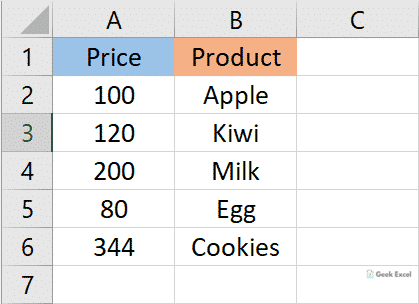
• Assuming that we have a list of products and their price amount.
• We are going to find the product whose price is more than 300 from the input range.
• In the below screenshot, you can see the example data.

Example data

• Then you need to enter the above-given formula in any cell. Here, we entered the formula in Cell E3.

Enter the formula

• After entering the formula, you need to press CTRL + SHIFT + Enter keys to get the result.
• Refer to the below screenshot.

Output

Closure:

In this post, we have described the steps to Lookup the Next Largest Value in Excel Office 365. Give your suggestions or feedback in the below comment box. Thanks for visiting Geek Excel!! Keep Learning!!

Keep Reading:

• Excel Formulas to Lookup Multiple Criteria with INDEX and MATCH!!
• Use Find & Replace Tool to Replace Text in Excel Office 365