Filter Data Based on Cell Value With Multiple Criteria in Excel Office 365!!

In this article, we are going to see how to Filter Data Based on Cell Value With Multiple Criteria in Excel Office 365 using Kutools. Get an official version of MS Excel from the following link: https://www.microsoft.com/en-in/microsoft-365/excel

Note: kutools for Excel has more than 180 features which are used to complete the difficult task with several clicks. If you want to use Kutools, you need to install it from Excel’s official website.

Filter Data Based on Cell Value with Criteria:

To filter data based on cell value with one criterion, do as follows.

• Let’s consider the below example data , we are going to filter it with the help of the Super Filter feature of Kutools.

Example data

• In this example, we will filter data based on the product = Apple.
• Go to the Kutools Plus Tab, select the Super Filter option.

Select the Super Filter option

• It will open the Super Filter pane on the right side of the worksheet.
• First, you need to select the Specified checkbox.
• Then, select the range that you want to filter using the browse button.
• Relationship drop-down list – You need to choose the OR of AND option.
• *Relationship in Group – * You can select the group relationship using this drop-down list.

Select the OR option

• Then, you need to click the horizontal line adjacent to the relationship AND. It will display some condition boxes, you need to select the criteria as you need.
• Then, you need to enter the condition that you want to use and click the OK button to add the condition.

Click the OK button

• Finally, you need to click the Filter button.

Click Filter option

• You can get the filtered result as shown in the below image.

Result

Steps to Filter Data Based on Cell Value with Multiple Criteria:

Here, we are going to see how to filter data based on the following criteria.

Criteria 1 : Product = Apple and Country = US

Criteria 2: Product = Grape and Quantity>30

The relationship between these two criteria is OR.

• The following screenshot has shown in the example range.

Sample data

• Now, you need to follow the below steps.
• On the Kutools Plus Tab, select the Super Filter option.

Select the Super Filter option

• It will open the Super Filter pane on the right side of the worksheet.
• Relationship drop-down list – You need to choose the OR option.
• Then, you can create the criteria as you need. Click Add Filter or Adding button to add a new condition group.
• Then, click the Filter option to filter the data.

Super Filter pane

• You will get the result as shown in the below image.

Output

Filter Data Based on Year/Month/Day/Week/Quarter:

If you want to filter rows based on year, month, day, week, or a quarter of the date, use the Super Filter function to complete the task.

• For example, we consider the below data given in the image.

Example data

• On the Kutools Plus Tab, select the Super Filter option.

Select the Super Filter option

• It will display the Super Filter pane on the right side of the worksheet.
• First, you need to select the Specified checkbox.
• Then, select the range that you want to filter using the browse button.
• Relationship drop-down list – You need to choose the OR or AND option.
• *Relationship in Group – * You can select the group relationship using this drop-down list.
• Then, you need to click the horizontal line adjacent to the relationship AND. It will display some condition boxes, you need to select the criteria as you need.
• Then, you need to enter the condition that you want to use and click the OK button to add the condition.

Super Filter pane

• At last, click the Filter button and the rows which date in quarter 4 have been filtered out as shown in the below image.

Output

• You can filter the data by month, year, day, week by applying the same steps.

Steps to Filter Data Based on Text Length/Number of Characters:

To filter data based on the text length/number of characters in Excel, follow the below steps.

• You need to activate the worksheet contains data that you want to filter.
• Refer to the below example worksheet with data.

Sample data

• Go to the Kutools Plus Tab, select the Super Filter option.

Select the Super Filter option

• It will show the Super Filter Dialog Box.
• Then, select the range that you want to filter using the browse button.
• Relationship drop-down list – You need to choose the OR of AND option.
• *Relationship in Group – * You can select the group relationship using this drop-down list.
• Then, you need to click the horizontal line adjacent to the relationship AND. It will display some condition boxes, you need to select the criteria as you need.
• Then, you need to enter the condition that you want to use and click the OK button to add the condition.
• Next, you need to click the Filter button.

Super Filter Dialog Box

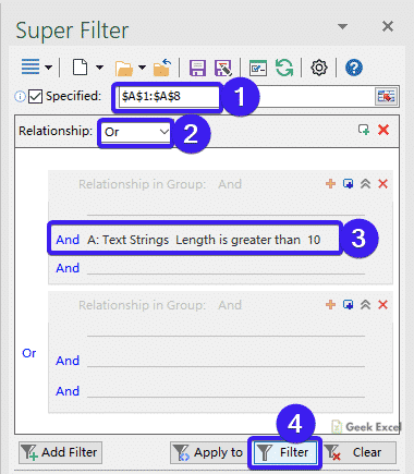
• You can see the rows which text length is greater than 10 characters have been filtered as shown in the below image.

Output

Filter Cell Text with Case Sensitive:

If you want to filter the rows in which the text string is only uppercase or lowercase, then follow the below instructions.

• Let’s consider the below example data.

Example

• On the Kutools Plus Tab, select the *Super Filter * option.

Select the Super Filter option

• It will show the Super Filter Dialog Box.
• Then, select the range that you want to filter using the browse button.
• Then, you need to click the horizontal line adjacent to the relationship AND.
• You need to choose the column name that you want to filter from the first & second drop-down lists and select the text format.
• Then, you need to choose the criteria from the third drop-down list.
• Then, you need to select the uppercase/lowercase text option to filter them (we choose UPPERCASE).
• Hit the OK button and click the Filter option.

Click Filter button

• You will get the filtered result as shown in the below image.

Result

Steps to Filter Cell Values with All Errors or One Specific Error:

To filter cell values with all errors or one specific error from the range in Excel, do as follows.

• You need to select the data that you want to filter.

Input

• On the Kutools Plus Tab, select the Super Filter option.

Select the Super Filter option

• It will open the Super Filter Dialog Box.
• You need to click the horizontal line beside the relationship AND.
• Then, choose the column name that you want to filter from the first drop-down list.
• You need to select the error that you want to filter from the second drop-down list.
• Then, select the criteria from the third drop-down list.
• Finally, you need to specify one choice you need and hit the OK button.

Super Filter

• Now, you need to click the Filter option to get the result as shown in the below screenshot.

Output

Save Filter Criteria as Scenario for Using Next Time:

• Click button to create a new filter settings scenario. If there are existing filter settings that are not saved, a dialog box will pop-out.

Kutools for Excel prompt box

• You need to click button to save your current filter settings. If the current filter settings are not saved before, a dialog box will display to name this new filter scenario.

Save Filter

• Click button to save the current filter settings to a new filter scenario.
• You can click button to close the current filter scenario.
• Click button to display the Open saved filter settings scenario dialog, then select a scenario in the right pane of the dialog to open it.

Click OK button

• You need to click to open the Manage filter settings scenarios dialog box. You can manage the scenarios of each scenario folder.

manage the scenarios

A Brief Summary:

In this article, you will easily understand the steps to Filter Data Based on Cell Value With Multiple Criteria in Excel Office 365 using Kutools. Leave your feedback in the comment section. Thanks for visiting Geek Excel. Keep Learning!

Read Ahead:

• How to Filter Cells by Background Color in Excel 365?
• Import Data from Another Worksheet or Text Files in Excel Office 365!!