Employee turnover analysis built using Python’s Scikit-Learn library.

In this article features, I showed the implementation of an employee turnover analysis that is built using Python’s Scikit-Learn library. In this article, I will use Logistic Regression and Random Forest Machine Learning algorithms.

At the end of this article, you would be able to choose the best algorithm for your future projects like Employee Turnover Prediction.

Definition Employee Turnover?

Employee Turnover or Employee Turnover ratio is the measurement of the total number of employees who leave an organization in a particular year. Employee Turnover Prediction understands that to predict whether an employee is going to leave the organization in the coming period.

A Company uses this predictive analysis to measure how many employees they will need if the potential employees will leave their organization. A company also uses this predictive analysis to make the workstation better for the employees by understanding the major reasons for the high turnover ratio.

Data Preprocessing system

Now let’s move into the data to learn further with this project on Employee Turnover Prediction. you can download the dataset, that I have used in this article from here. Link

import pandas as pd
hr = pd.read_csv('HR_comma_sep.csv')
col_names = hr.columns.tolist()
print("Column names:")
print(col_names)
print("\nSample data:")
hr.head()

Output:

Rename column name from “sales” to “department”:

hr=hr.rename(columns = {'sales':'department'})

Our data is pretty clean, with no missing values, so let’s move further and see how many employees work in the organization:

hr.shape

The “left” column is the outcome variable recording one and 0. 1 for employees who left the company and 0 for those who didn't. The department column of the dataset has many categories, and we need to reduce the categories for better modeling. Let’s see all the categories of the department column:

hr['department'].unique()

Output:

Let’s add all the “technical”, “support” and “IT” columns into one column to make our analysis easier.

import numpy as np
hr['department']=np.where(hr['department'] =='support', 'technical', hr['department'])
hr['department']=np.where(hr['department'] =='IT', 'technical', hr['department'])

Creating Variables for Categorical Variables

As there are two categorical variables (department, salary) in the dataset and they need to be converted to dummy variables before they can be used for modeling.

cat_vars=['department','salary']
for var in cat_vars:
    cat_list='var'+'_'+var
    cat_list = pd.get_dummies(hr[var], prefix=var)
    hr1=hr.join(cat_list)
    hr=hr1

Now the actual variables need to be removed after the dummy variable has been created. Column names after creating dummy variables for categorical variables:

hr.drop(hr.columns[[8, 9]], axis=1, inplace=True)
hr.columns.values

Output:

The outcome variable is “left”, and all the other variables are predictors.

hr_vars=hr.columns.values.tolist()
y=['left']
X=[i for i in hr_vars if i not in y]

Feature Selection for Employee Turnover Prediction

Let’s use the feature selection method to decide which variables are the best option that can predict employee turnover with great accuracy. There are a total of 18 columns in X, and now let’s see how we can select about 10 from them:

from sklearn.feature_selection import RFE
from sklearn.linear_model import LogisticRegression
model = LogisticRegression()
rfe = RFE(model, 10)
rfe = rfe.fit(hr[X], hr[y])
print(rfe.support_)
print(rfe.ranking_)

Output:

You can see that or feature selection chose the 10 variables for us, which are marked True in the support_ array and marked with a choice “1” in the ranking array. Now let's have a look at these columns:

cols=['satisfaction_level', 'last_evaluation', 'time_spend_company', 'Work_accident', 'promotion_last_5years', 
      'department_RandD', 'department_hr', 'department_management', 'salary_high', 'salary_low'] 
X=hr[cols]
y=hr['left']

Logistic Regression Model to Predict Employee Turnover

from sklearn.model_selection import train_test_split
X_train, X_test, y_train, y_test = train_test_split(X, y, test_size=0.3, random_state=0)
from sklearn.linear_model import LogisticRegression
from sklearn import metrics
logreg = LogisticRegression()
logreg.fit(X_train, y_train)

Output:

Let’s check the accuracy of our logistic regression model.

from sklearn.metrics import accuracy_score
print('Logistic regression accuracy: {:.3f}'.format(accuracy_score(y_test, logreg.predict(X_test))))

Output:

Random Forest Classification Model

from sklearn.ensemble import RandomForestClassifier
rf = RandomForestClassifier()
rf.fit(X_train, y_train)

Output:

Now let’s check the accuracy of our Random Forest Classification Model:

print('Random Forest Accuracy: {:.3f}'.format(accuracy_score(y_test, rf.predict(X_test))))

Output:

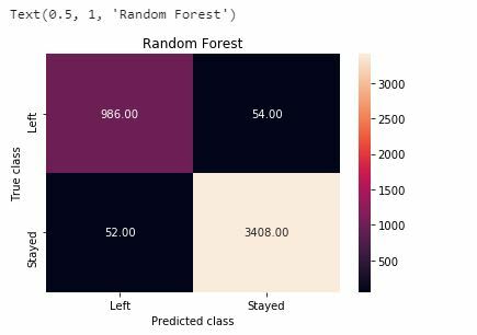
Confusion Matrix for our Machine Learning Models

Now I will construct a confusion matrix to visualize predictions made by our classifier and evaluate the accuracy of our machine learning classification.

Random Forest

from sklearn.metrics import classification_report
print(classification_report(y_test, rf.predict(X_test)))

Output:

import matplotlib
import matplotlib.pyplot as plt
y_pred = rf.predict(X_test)
from sklearn.metrics import confusion_matrix
import seaborn as sns
forest_cm = metrics.confusion_matrix(y_pred, y_test, [1,0])
sns.heatmap(forest_cm, annot=True, fmt='.2f',xticklabels = ["Left", "Stayed"] , yticklabels = ["Left", "Stayed"] )
plt.ylabel('True class')
plt.xlabel('Predicted class')
plt.title('Random Forest')

Output:

Logistic Regression

print(classification_report(y_test, logreg.predict(X_test)))

Output:

import matplotlib
import matplotlib.pyplot as plt
logreg_y_pred = logreg.predict(X_test)
logreg_cm = metrics.confusion_matrix(logreg_y_pred, y_test, [1,0])
sns.heatmap(logreg_cm, annot=True, fmt='.2f',xticklabels = ["Left", "Stayed"] , yticklabels = ["Left", "Stayed"] )
plt.ylabel('True class')
plt.xlabel('Predicted class')
plt.title('Logistic Regression')

Output:

Employee Turnover Prediction Curve

import matplotlib
import matplotlib.pyplot as plt
from sklearn.metrics import roc_auc_score
from sklearn.metrics import roc_curve
logit_roc_auc = roc_auc_score(y_test, logreg.predict(X_test))
fpr, tpr, thresholds = roc_curve(y_test, logreg.predict_proba(X_test)[:,1])
rf_roc_auc = roc_auc_score(y_test, rf.predict(X_test))
rf_fpr, rf_tpr, rf_thresholds = roc_curve(y_test, rf.predict_proba(X_test)[:,1])
plt.figure()
plt.plot(fpr, tpr, label='Logistic Regression (area = %0.2f)' % logit_roc_auc)
plt.plot(rf_fpr, rf_tpr, label='Random Forest (area = %0.2f)' % rf_roc_auc)
plt.plot([0, 1], [0, 1],'r--')
plt.xlim([0.0, 1.0])
plt.ylim([0.0, 1.05])
plt.xlabel('False Positive Rate')
plt.ylabel('True Positive Rate')
plt.title('Receiver operating characteristic')
plt.legend(loc="lower right")
plt.show()

Output:

The receiver operating characteristic (ROC) curve is a standard tool used with binary classifiers. The red dotted line represents the ROC curve of a purely random classifier; a good classifier stays as far away from that line as possible (toward the top-left corner).
So, as we can see that the Random Forest Model has proven to be more useful in the prediction of employee turnover, now let’s have a look at the feature importance of our random forest classification model.

feature_labels = np.array(['satisfaction_level', 'last_evaluation', 'time_spend_company', 'Work_accident', 'promotion_last_5years', 
      'department_RandD', 'department_hr', 'department_management', 'salary_high', 'salary_low'])
importance = rf.feature_importances_
feature_indexes_by_importance = importance.argsort()
for index in feature_indexes_by_importance:
    print('{}-{:.2f}%'.format(feature_labels[index], (importance[index] *100.0)))

Output:

According to our Random Forest classification model, the above aspects show the most important features which will influence whether an employee will leave the company, in ascending order.