
Fundamental Data Structures in JavaScript
(and a bit of python pseudo code)
Table Of Contents:
- Fundamental Data Structures in JavaScript
- Table Of Contents:
-
Resuorces:
- Data Structures & Algorithms Resource List Part 1
- Guess the author of the following quotes:
- Update:
- Algorithms
- Data Structures:
- A simple to follow guide to Lists Stacks and Queues, with animated gifs, diagrams, and code examples
- Linked Lists
- What is a Linked List?
- Types of Linked Lists
- Linked List Methods
- Time and Space Complexity Analysis
- Time Complexity — Access and Search
- Time Complexity — Insertion and Deletion
- Space Complexity
- Stacks and Queues
- What is a Stack?
- What is a Queue?
- Stack and Queue Properties
- Time and Space Complexity Analysis
- When should we use Stacks and Queues?
-
Graphs:
- Graph Data Structure Interview Questions At A Glance
- Graphs
- Questions
- Graph Representations
- Adjacency List
- Adjacency Matrix
- Tradeoffs
- Breadth-First Search
- Applications of BFS
- Coloring BFS
- BFS Pseudocode
- BFS Steps
- Depth-First Search
- Applications of DFS
- DFS Pseudocode
- DFS Steps
- Connected Components
- Uses
- How to find connected componnents
- Bonus Python Question
- This Bellman-Ford Code is for determination whether we can get
- shortest path from given graph or not for single-source shortest-paths problem.
- In other words, if given graph has any negative-weight cycle that is reachable
- from the source, then it will give answer False for "no solution exits".
- For argument graph, it should be a dictionary type
-
such as
- Review of Concepts
- Undirected Graph
- Types
- Dense Graph
- Sparse Graph
- Weighted Graph
- Directed Graph
- Undirected Graph
- Node Class
- Adjacency Matrix
- Adjacency List
- Data Structures… Under The Hood
- Data Structures Reference
- Array
- Linked List
- Queue
- Stack
- Tree
- Binary Search Tree
- Binary Search Tree
- Graph
- Heap
- Adjacency list
- Adjacency matrix
- Arrays
- Pointers
- Linked lists
- Doubly Linked Lists
- Not cache-friendly
- Hash tables
- Breadth-First Search (BFS) and Breadth-First Traversal
- Binary Search Tree
- Graph Data Structure: Directed, Acyclic, etc
- Binary numbers
-
Implementations
- Resources (article content below):
- space
- time
- Several operations
- Dependent on data
- Big O notation
- The Array data structure
- Definition
- 2. Objects
- The Hash Table
- Definition
- The Set
- Sets
- Definition
- The Singly Linked List
- Definition
- The Doubly Linked List
- Definition
- The Stack
- Definition
- The Queue
- Definition
- The Tree
- Definition
- The Graph
- Definition
- Cycle Visual
- Ways to Reference Graph Nodes
- Node Class
- Adjacency Matrix
- Adjacency List
- Code Examples
- Basic Graph Class
- Node Class Examples
- Traversal Examples
- With Adjacency List
- Memoization & Tabulation (Dynamic Programming)
- Practice:
Resuorces:
_**
🏐⇒⇒⇒Click Here To Expand⇐⇐⇐🏐**_
Data Structures & Algorithms Resource List Part 1
Guess the author of the following quotes:

> Talk is cheap. Show me the code.
> Software is like sex: it's better when it's free.
> Microsoft isn't evil, they just make really crappy operating systems.

Update:
- The Framework for Learning Algorithms and intense problem solving exercises
- Algs4: Recommended book for Learning Algorithms and Data Structures
- An analysis of Dynamic Programming
- Dynamic Programming Q&A — What is Optimal Substructure
- The Framework for Backtracking Algorithm
- Binary Search in Detail: I wrote a Poem
- The Sliding Window Technique
- Difference Between Process and Thread in Linux
- Some Good Online Practice Platforms
- Dynamic Programming in Details
- Dynamic Programming Q&A — What is Optimal Substructure
- Classic DP: Longest Common Subsequence
- Classic DP: Edit Distance
- Classic DP: Super Egg
- Classic DP: Super Egg (Advanced Solution)
- The Strategies of Subsequence Problem
- Classic DP: Game Problems
- Greedy: Interval Scheduling
- KMP Algorithm In Detail
- A solution to all Buy Time to Buy and Sell Stock Problems
- A solution to all House Robber Problems
- 4 Keys Keyboard
- Regular Expression
- Longest Increasing Subsequence
- The Framework for Learning Algorithms and intense problem solving exercises
- Algs4: Recommended book for Learning Algorithms and Data Structures
- Binary Heap and Priority Queue
- LRU Cache Strategy in Detail
- Collections of Binary Search Operations
- Special Data Structure: Monotonic Stack
- Special Data Structure: Monotonic Stack
- Design Twitter
- Reverse Part of Linked List via Recursion
- Queue Implement Stack/Stack implement Queue
- My Way to Learn Algorithm
- The Framework of Backtracking Algorithm
- Binary Search in Detail
- Backtracking Solve Subset/Permutation/Combination
- Diving into the technical parts of Double Pointers
- Sliding Window Technique
- The Core Concept of TwoSum Problems
- Common Bit Manipulations
- Breaking down a Complicated Problem: Implement a Calculator
- Pancake Sorting Algorithm
- Prefix Sum: Intro and Concept
- String Multiplication
- FloodFill Algorithm in Detail
- Interval Scheduling: Interval Merging
- Interval Scheduling: Intersections of Intervals
- Russian Doll Envelopes Problem
- A collection of counter-intuitive Probability Problems
- Shuffle Algorithm
- Recursion In Detail
- How to Implement LRU Cache
- How to Find Prime Number Efficiently
- How to Calculate Minimium Edit Distance
- How to use Binary Search
- How to efficiently solve Trapping Rain Water Problem
- How to Remove Duplicates From Sorted Array
- How to Find Longest Palindromic Substring
- How to Reverse Linked List in K Group
- How to Check the Validation of Parenthesis
- How to Find Missing Element
- How to Find Duplicates and Missing Elements
- How to Check Palindromic LinkedList
- How to Pick Elements From an Infinite Arbitrary Sequence
- How to Schedule Seats for Students
- Union-Find Algorithm in Detail
- Union-Find Application
- Problems that can be solved in one line
- Find Subsequence With Binary Search
- Difference Between Process and Thread in Linux
- You Must Know About Linux Shell
- You Must Know About Cookie and Session
- Cryptology Algorithm
- Some Good Online Practice Platforms
Algorithms
- 100 days of algorithms
- Algorithms — Solved algorithms and data structures problems in many languages.
- Algorithms by Jeff Erickson (Code) (HN)
- Top algos/DS to learn
- Some neat algorithms
- Mathematical Proof of Algorithm Correctness and Efficiency (2019)
- Algorithm Visualizer — Interactive online platform that visualizes algorithms from code.
- Algorithms for Optimization book
- Collaborative book on algorithms (Code)
- Algorithms in C by Robert Sedgewick
- Algorithm Design Manual
- MIT Introduction to Algorithms course (2011)
- How to implement an algorithm from a scientific paper (2012)
- Quadsort — Stable non-recursive merge sort named quadsort.
- System design algorithms — Algorithms you should know before system design.
- Algorithms Design book
- Think Complexity
- All Algorithms implemented in Rust
- Solutions to Introduction to Algorithms book (Code)
- Maze Algorithms (2011) (HN)
- Algorithmic Design Paradigms book (Code)
- Words and buttons Online Blog (Code)
- Algorithms animated
- Cache Oblivious Algorithms (2020) (HN)
- You could have invented fractional cascading (2012)
- Guide to learning algorithms through LeetCode (Code) (HN)
- How hard is unshuffling a string?
- Optimization Algorithms on Matrix Manifolds
- Problem Solving with Algorithms and Data Structures (HN) (PDF)
- Algorithms implemented in Python
- Algorithms implemented in JavaScript
- Algorithms & Data Structures in Java
- Wolfsort — Stable adaptive hybrid radix / merge sort.
- Evolutionary Computation Bestiary — Bestiary of evolutionary, swarm and other metaphor-based algorithms.
- Elements of Programming book — Decomposing programs into a system of algorithmic components. (Review) (HN) (Lobsters)
- Competitive Programming Algorithms
- CPP/C — C/C++ algorithms/DS problems.
- How to design an algorithm (2018)
- CSE 373 — Introduction to Algorithms, by Steven Skiena (2020)
- Computer Algorithms II course (2020)
- Improving Binary Search by Guessing (2019)
- The case for a learned sorting algorithm (2020) (HN)
- Elementary Algorithms — Introduces elementary algorithms and data structures. Includes side-by-side comparisons of purely functional realization and their imperative counterpart.
- Combinatorics Algorithms for Coding Interviews (2018)
- Algorithms written in different programming languages (Web)
- Solving the Sequence Alignment problem in Python (2020)
- The Sound of Sorting — Visualization and "Audibilization" of Sorting Algorithms. (Web)
- Miniselect: Practical and Generic Selection Algorithms (2020)
- The Slowest Quicksort (2019)
- Functional Algorithm Design (2020)
- Algorithms To Live By — Book Notes
- Numerical Algorithms (2015)
- Using approximate nearest neighbor search in real world applications (2020)
- In search of the fastest concurrent Union-Find algorithm (2019)
- Computer Science 521 Advanced Algorithm Design

Data Structures:
- Data Structures and Algorithms implementation in Go
- Which algorithms/data structures should I "recognize" and know by name?
- Dictionary of Algorithms and Data Structures
- Phil's Data Structure Zoo
- The Periodic Table of Data Structures (HN)
- Data Structure Visualizations (HN)
- Data structures to name-drop when you want to sound smart in an interview
- On lists, cache, algorithms, and microarchitecture (2019)
- Topics in Advanced Data Structures (2019) (HN)
## A simple to follow guide to Lists Stacks and Queues, with animated gifs, diagrams, and code examples

Linked Lists
 In the university setting, it's common for Linked Lists to appear early on in an undergraduate's Computer Science coursework. While they don't always have the most practical real-world applications in industry, Linked Lists make for an important and effective educational tool in helping develop a student's mental model on what data structures actually are to begin with.
Linked lists are simple. They have many compelling, reoccurring edge cases to consider that emphasize to the student the need for care and intent while implementing data structures. They can be applied as the underlying data structure while implementing a variety of other prevalent abstract data types, such as Lists, Stacks, and Queues, and they have a level of versatility high enough to clearly illustrate the value of the Object Oriented Programming paradigm.
They also come up in software engineering interviews quite often.
In the university setting, it's common for Linked Lists to appear early on in an undergraduate's Computer Science coursework. While they don't always have the most practical real-world applications in industry, Linked Lists make for an important and effective educational tool in helping develop a student's mental model on what data structures actually are to begin with.
Linked lists are simple. They have many compelling, reoccurring edge cases to consider that emphasize to the student the need for care and intent while implementing data structures. They can be applied as the underlying data structure while implementing a variety of other prevalent abstract data types, such as Lists, Stacks, and Queues, and they have a level of versatility high enough to clearly illustrate the value of the Object Oriented Programming paradigm.
They also come up in software engineering interviews quite often.

What is a Linked List?
A Linked List data structure represents a linear sequence of "vertices" (or "nodes"), and tracks three important properties.
Linked List Properties:
 The data being tracked by a particular Linked List does not live inside the Linked List instance itself. Instead, each vertex is actually an instance of an even simpler, smaller data structure, often referred to as a "Node".
Depending on the type of Linked List (there are many), Node instances track some very important properties as well.
**Linked List Node Properties:**
The data being tracked by a particular Linked List does not live inside the Linked List instance itself. Instead, each vertex is actually an instance of an even simpler, smaller data structure, often referred to as a "Node".
Depending on the type of Linked List (there are many), Node instances track some very important properties as well.
**Linked List Node Properties:**
 Property Description `value`: The actual value this node represents.`next`The next node in the list (relative to this node).`previous`The previous node in the list (relative to this node).
**NOTE:** The `previous` property is for Doubly Linked Lists only!
Linked Lists contain _ordered_ data, just like arrays. The first node in the list is, indeed, first. From the perspective of the very first node in the list, the _next_ node is the second node. From the perspective of the second node in the list, the _previous_ node is the first node, and the _next_ node is the third node. And so it goes.
#### "So…this sounds a lot like an Array…"
Admittedly, this does _sound_ a lot like an Array so far, and that's because Arrays and Linked Lists are both implementations of the List ADT. However, there is an incredibly important distinction to be made between Arrays and Linked Lists, and that is how they _physically store_ their data. (As opposed to how they _represent_ the order of their data.)
Recall that Arrays contain _contiguous_ data. Each element of an array is actually stored _next to_ it's neighboring element _in the actual hardware of your machine_, in a single continuous block in memory.
_An Array's contiguous data being stored in a continuous block of addresses in memory._
Unlike Arrays, Linked Lists contain _non-contiguous_ data. Though Linked Lists _represent_ data that is ordered linearly, that mental model is just that — an interpretation of the _representation_ of information, not reality.
In reality, in the actual hardware of your machine, whether it be in disk or in memory, a Linked List's Nodes are not stored in a single continuous block of addresses. Rather, Linked List Nodes live at randomly distributed addresses throughout your machine! The only reason we know which node comes next in the list is because we've assigned its reference to the current node's `next` pointer.
_A Singly Linked List's non-contiguous data (Nodes) being stored at randomly distributed addresses in memory._
For this reason, Linked List Nodes have _no indices_, and no _random access_. Without random access, we do not have the ability to look up an individual Linked List Node in constant time. Instead, to find a particular Node, we have to start at the very first Node and iterate through the Linked List one node at a time, checking each Node's _next_ Node until we find the one we're interested in.
So when implementing a Linked List, we actually must implement both the Linked List class _and_ the Node class. Since the actual data lives in the Nodes, it's simpler to implement the Node class first.
### Types of Linked Lists
There are four flavors of Linked List you should be familiar with when walking into your job interviews.
**Linked List Types:**
Property Description `value`: The actual value this node represents.`next`The next node in the list (relative to this node).`previous`The previous node in the list (relative to this node).
**NOTE:** The `previous` property is for Doubly Linked Lists only!
Linked Lists contain _ordered_ data, just like arrays. The first node in the list is, indeed, first. From the perspective of the very first node in the list, the _next_ node is the second node. From the perspective of the second node in the list, the _previous_ node is the first node, and the _next_ node is the third node. And so it goes.
#### "So…this sounds a lot like an Array…"
Admittedly, this does _sound_ a lot like an Array so far, and that's because Arrays and Linked Lists are both implementations of the List ADT. However, there is an incredibly important distinction to be made between Arrays and Linked Lists, and that is how they _physically store_ their data. (As opposed to how they _represent_ the order of their data.)
Recall that Arrays contain _contiguous_ data. Each element of an array is actually stored _next to_ it's neighboring element _in the actual hardware of your machine_, in a single continuous block in memory.
_An Array's contiguous data being stored in a continuous block of addresses in memory._
Unlike Arrays, Linked Lists contain _non-contiguous_ data. Though Linked Lists _represent_ data that is ordered linearly, that mental model is just that — an interpretation of the _representation_ of information, not reality.
In reality, in the actual hardware of your machine, whether it be in disk or in memory, a Linked List's Nodes are not stored in a single continuous block of addresses. Rather, Linked List Nodes live at randomly distributed addresses throughout your machine! The only reason we know which node comes next in the list is because we've assigned its reference to the current node's `next` pointer.
_A Singly Linked List's non-contiguous data (Nodes) being stored at randomly distributed addresses in memory._
For this reason, Linked List Nodes have _no indices_, and no _random access_. Without random access, we do not have the ability to look up an individual Linked List Node in constant time. Instead, to find a particular Node, we have to start at the very first Node and iterate through the Linked List one node at a time, checking each Node's _next_ Node until we find the one we're interested in.
So when implementing a Linked List, we actually must implement both the Linked List class _and_ the Node class. Since the actual data lives in the Nodes, it's simpler to implement the Node class first.
### Types of Linked Lists
There are four flavors of Linked List you should be familiar with when walking into your job interviews.
**Linked List Types:**
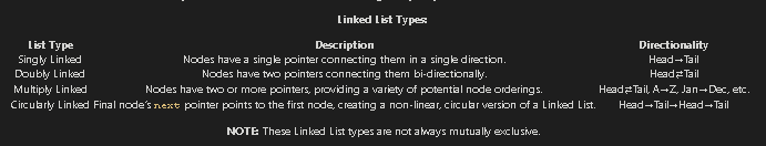 ***Note:****These Linked List types are not always mutually exclusive.*
For instance:
- Any type of Linked List can be implemented Circularly (e.g. A Circular Doubly Linked List).
- A Doubly Linked List is actually just a special case of a Multiply Linked List.
You are most likely to encounter Singly and Doubly Linked Lists in your upcoming job search, so we are going to focus exclusively on those two moving forward. However, in more senior level interviews, it is very valuable to have some familiarity with the other types of Linked Lists. Though you may not actually code them out, _you will win extra points by illustrating your ability to weigh the tradeoffs of your technical decisions_ by discussing how your choice of Linked List type may affect the efficiency of the solutions you propose.
### Linked List Methods
***Note:****These Linked List types are not always mutually exclusive.*
For instance:
- Any type of Linked List can be implemented Circularly (e.g. A Circular Doubly Linked List).
- A Doubly Linked List is actually just a special case of a Multiply Linked List.
You are most likely to encounter Singly and Doubly Linked Lists in your upcoming job search, so we are going to focus exclusively on those two moving forward. However, in more senior level interviews, it is very valuable to have some familiarity with the other types of Linked Lists. Though you may not actually code them out, _you will win extra points by illustrating your ability to weigh the tradeoffs of your technical decisions_ by discussing how your choice of Linked List type may affect the efficiency of the solutions you propose.
### Linked List Methods

Linked Lists are great foundation builders when learning about data structures because they share a number of similar methods (and edge cases) with many other common data structures. You will find that many of the concepts discussed here will repeat themselves as we dive into some of the more complex non-linear data structures later on, like Trees and Graphs.
Time and Space Complexity Analysis
Before we begin our analysis, here is a quick summary of the Time and Space constraints of each Linked List Operation. The complexities below apply to both Singly and Doubly Linked Lists:

Before moving forward, see if you can reason to yourself why each operation has the time and space complexity listed above!
Time Complexity — Access and Search
Scenarios
- We have a Linked List, and we'd like to find the 8th item in the list.
- We have a Linked List of sorted alphabet letters, and we'd like to see if the letter "Q" is inside that list.
Discussion
Unlike Arrays, Linked Lists Nodes are not stored contiguously in memory, and thereby do not have an indexed set of memory addresses at which we can quickly lookup individual nodes in constant time. Instead, we must begin at the head of the list (or possibly at the tail, if we have a Doubly Linked List), and iterate through the list until we arrive at the node of interest.
In Scenario 1, we'll know we're there because we've iterated 8 times. In Scenario 2, we'll know we're there because, while iterating, we've checked each node's value and found one that matches our target value, "Q".
In the worst case scenario, we may have to traverse the entire Linked List until we arrive at the final node. This makes both Access & Search Linear Time operations.
Time Complexity — Insertion and Deletion
Scenarios
- We have an empty Linked List, and we'd like to insert our first node.
- We have a Linked List, and we'd like to insert or delete a node at the Head or Tail.
- We have a Linked List, and we'd like to insert or delete a node from somewhere in the middle of the list.
Discussion
Since we have our Linked List Nodes stored in a non-contiguous manner that relies on pointers to keep track of where the next and previous nodes live, Linked Lists liberate us from the linear time nature of Array insertions and deletions. We no longer have to adjust the position at which each node/element is stored after making an insertion at a particular position in the list. Instead, if we want to insert a new node at position i, we can simply:
- Create a new node.
- Set the new node's
nextandpreviouspointers to the nodes that live at positionsiandi - 1, respectively. - Adjust the
nextpointer of the node that lives at positioni - 1to point to the new node. - Adjust the
previouspointer of the node that lives at positionito point to the new node.
And we're done, in Constant Time. No iterating across the entire list necessary.
"But hold on one second," you may be thinking. "In order to insert a new node in the middle of the list, don't we have to lookup its position? Doesn't that take linear time?!"
Yes, it is tempting to call insertion or deletion in the middle of a Linked List a linear time operation since there is lookup involved. However, it's usually the case that you'll already have a reference to the node where your desired insertion or deletion will occur.
For this reason, we separate the Access time complexity from the Insertion/Deletion time complexity, and formally state that Insertion and Deletion in a Linked List are Constant Time across the board.
Note: Without a reference to the node at which an insertion or deletion will occur, due to linear time lookup, an insertion or deletion in the middle of a Linked List will still take Linear Time, sum total.
Space Complexity
Scenarios
- We're given a Linked List, and need to operate on it.
- We've decided to create a new Linked List as part of strategy to solve some problem.
Discussion
It's obvious that Linked Lists have one node for every one item in the list, and for that reason we know that Linked Lists take up Linear Space in memory. However, when asked in an interview setting what the Space Complexity of your solution to a problem is, it's important to recognize the difference between the two scenarios above.
In Scenario 1, we are not creating a new Linked List. We simply need to operate on the one given. Since we are not storing a new node for every node represented in the Linked List we are provided, our solution is not necessarily linear in space.
In Scenario 2, we are creating a new Linked List. If the number of nodes we create is linearly correlated to the size of our input data, we are now operating in Linear Space.
*Note**: Linked Lists can be traversed both iteratively and recursively. If you choose to traverse a Linked List recursively, there will be a recursive function call added to the call stack for every node in the Linked List. Even if you're provided the Linked List, as in Scenario 1, you will still use Linear Space in the call stack, and that counts.*
Stacks and Queues
Stacks and Queues aren't really "data structures" by the strict definition of the term. The more appropriate terminology would be to call them abstract data types (ADTs), meaning that their definitions are more conceptual and related to the rules governing their user-facing behaviors rather than their core implementations.
For the sake of simplicity, we'll refer to them as data structures and ADTs interchangeably throughout the course, but the distinction is an important one to be familiar with as you level up as an engineer.
Now that that's out of the way, Stacks and Queues represent a linear collection of nodes or values. In this way, they are quite similar to the Linked List data structure we discussed in the previous section. In fact, you can even use a modified version of a Linked List to implement each of them. (Hint, hint.)
These two ADTs are similar to each other as well, but each obey their own special rule regarding the order with which Nodes can be added and removed from the structure.
Since we've covered Linked Lists in great length, these two data structures will be quick and easy. Let's break them down individually in the next couple of sections.
What is a Stack?
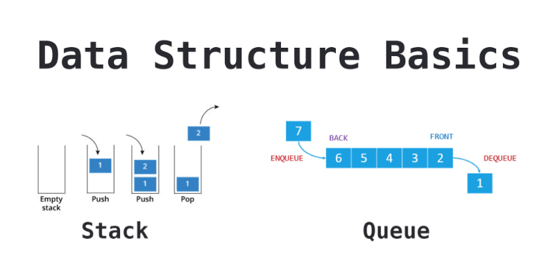
Stacks are a Last In First Out (LIFO) data structure. The last Node added to a stack is always the first Node to be removed, and as a result, the first Node added is always the last Node removed.
The name Stack actually comes from this characteristic, as it is helpful to visualize the data structure as a vertical stack of items. Personally, I like to think of a Stack as a stack of plates, or a stack of sheets of paper. This seems to make them more approachable, because the analogy relates to something in our everyday lives.
If you can imagine adding items to, or removing items from, a Stack of…literally anything…you'll realize that every (sane) person naturally obeys the LIFO rule.
We add things to the top of a stack. We remove things from the top of a stack. We never add things to, or remove things from, the bottom of the stack. That's just crazy.
Note: We can use JavaScript Arrays to implement a basic stack. Array#push adds to the top of the stack and Array#pop will remove from the top of the stack. In the exercise that follows, we'll build our own Stack class from scratch (without using any arrays). In an interview setting, your evaluator may be okay with you using an array as a stack.
What is a Queue?
Queues are a First In First Out (FIFO) data structure. The first Node added to the queue is always the first Node to be removed.
The name Queue comes from this characteristic, as it is helpful to visualize this data structure as a horizontal line of items with a beginning and an end. Personally, I like to think of a Queue as the line one waits on for an amusement park, at a grocery store checkout, or to see the teller at a bank.
If you can imagine a queue of humans waiting…again, for literally anything…you'll realize that most people (the civil ones) naturally obey the FIFO rule.
People add themselves to the back of a queue, wait their turn in line, and make their way toward the front. People exit from the front of a queue, but only when they have made their way to being first in line.
We never add ourselves to the front of a queue (unless there is no one else in line), otherwise we would be "cutting" the line, and other humans don't seem to appreciate that.
Note: We can use JavaScript Arrays to implement a basic queue. Array#push adds to the back (enqueue) and Array#shift will remove from the front (dequeue). In the exercise that follows, we'll build our own Queue class from scratch (without using any arrays). In an interview setting, your evaluator may be okay with you using an array as a queue.
Stack and Queue Properties
Stacks and Queues are so similar in composition that we can discuss their properties together. They track the following three properties:
Stack Properties | Queue Properties:
 Notice that rather than having a `head` and a `tail` like Linked Lists, Stacks have a `top`, and Queues have a `front` and a `back` instead. Stacks don't have the equivalent of a `tail` because you only ever push or pop things off the top of Stacks. These properties are essentially the same; pointers to the end points of the respective List ADT where important actions way take place. The differences in naming conventions are strictly for human comprehension.
--------
Similarly to Linked Lists, the values stored inside a Stack or a Queue are actually contained within Stack Node and Queue Node instances. Stack, Queue, and Singly Linked List Nodes are all identical, but just as a reminder and for the sake of completion, these List Nodes track the following two properties:
### Time and Space Complexity Analysis
Before we begin our analysis, here is a quick summary of the Time and Space constraints of each Stack Operation.
Data Structure Operation Time Complexity (Avg)Time Complexity (Worst)Space Complexity (Worst)Access`Θ(n)O(n)O(n)`Search`Θ(n)O(n)O(n)`Insertion`Θ(1)O(1)O(n)`Deletion`Θ(1)O(1)O(n)`
Before moving forward, see if you can reason to yourself why each operation has the time and space complexity listed above!
#### Time Complexity — Access and Search
When the Stack ADT was first conceived, its inventor definitely did not prioritize searching and accessing individual Nodes or values in the list. The same idea applies for the Queue ADT. There are certainly better data structures for speedy search and lookup, and if these operations are a priority for your use case, it would be best to choose something else!
Search and Access are both linear time operations for Stacks and Queues, and that shouldn't be too unclear. Both ADTs are nearly identical to Linked Lists in this way. The only way to find a Node somewhere in the middle of a Stack or a Queue, is to start at the `top` (or the `back`) and traverse downward (or forward) toward the `bottom` (or `front`) one node at a time via each Node's `next` property.
This is a linear time operation, O(n).
#### Time Complexity — Insertion and Deletion
For Stacks and Queues, insertion and deletion is what it's all about. If there is one feature a Stack absolutely must have, it's constant time insertion and removal to and from the `top` of the Stack (FIFO). The same applies for Queues, but with insertion occurring at the `back` and removal occurring at the `front` (LIFO).
Think about it. When you add a plate to the top of a stack of plates, do you have to iterate through all of the other plates first to do so? Of course not. You simply add your plate to the top of the stack, and that's that. The concept is the same for removal.
Therefore, Stacks and Queues have constant time Insertion and Deletion via their `push` and `pop` or `enqueue` and `dequeue` methods, O(1).
#### Space Complexity
The space complexity of Stacks and Queues is very simple. Whether we are instantiating a new instance of a Stack or Queue to store a set of data, or we are using a Stack or Queue as part of a strategy to solve some problem, Stacks and Queues always store one Node for each value they receive as input.
For this reason, we always consider Stacks and Queues to have a linear space complexity, O(n).
### When should we use Stacks and Queues?
At this point, we've done a lot of work understanding the ins and outs of Stacks and Queues, but we still haven't really discussed what we can use them for. The answer is actually…a lot!
For one, Stacks and Queues can be used as intermediate data structures while implementing some of the more complicated data structures and methods we'll see in some of our upcoming sections.
For example, the implementation of the breadth-first Tree traversal algorithm takes advantage of a Queue instance, and the depth-first Graph traversal algorithm exploits the benefits of a Stack instance.
Additionally, Stacks and Queues serve as the essential underlying data structures to a wide variety of applications you use all the time. Just to name a few:
# Graphs:
### Graph Data Structure Interview Questions At A Glance
> Because they're just about the most important data structure there is.
Notice that rather than having a `head` and a `tail` like Linked Lists, Stacks have a `top`, and Queues have a `front` and a `back` instead. Stacks don't have the equivalent of a `tail` because you only ever push or pop things off the top of Stacks. These properties are essentially the same; pointers to the end points of the respective List ADT where important actions way take place. The differences in naming conventions are strictly for human comprehension.
--------
Similarly to Linked Lists, the values stored inside a Stack or a Queue are actually contained within Stack Node and Queue Node instances. Stack, Queue, and Singly Linked List Nodes are all identical, but just as a reminder and for the sake of completion, these List Nodes track the following two properties:
### Time and Space Complexity Analysis
Before we begin our analysis, here is a quick summary of the Time and Space constraints of each Stack Operation.
Data Structure Operation Time Complexity (Avg)Time Complexity (Worst)Space Complexity (Worst)Access`Θ(n)O(n)O(n)`Search`Θ(n)O(n)O(n)`Insertion`Θ(1)O(1)O(n)`Deletion`Θ(1)O(1)O(n)`
Before moving forward, see if you can reason to yourself why each operation has the time and space complexity listed above!
#### Time Complexity — Access and Search
When the Stack ADT was first conceived, its inventor definitely did not prioritize searching and accessing individual Nodes or values in the list. The same idea applies for the Queue ADT. There are certainly better data structures for speedy search and lookup, and if these operations are a priority for your use case, it would be best to choose something else!
Search and Access are both linear time operations for Stacks and Queues, and that shouldn't be too unclear. Both ADTs are nearly identical to Linked Lists in this way. The only way to find a Node somewhere in the middle of a Stack or a Queue, is to start at the `top` (or the `back`) and traverse downward (or forward) toward the `bottom` (or `front`) one node at a time via each Node's `next` property.
This is a linear time operation, O(n).
#### Time Complexity — Insertion and Deletion
For Stacks and Queues, insertion and deletion is what it's all about. If there is one feature a Stack absolutely must have, it's constant time insertion and removal to and from the `top` of the Stack (FIFO). The same applies for Queues, but with insertion occurring at the `back` and removal occurring at the `front` (LIFO).
Think about it. When you add a plate to the top of a stack of plates, do you have to iterate through all of the other plates first to do so? Of course not. You simply add your plate to the top of the stack, and that's that. The concept is the same for removal.
Therefore, Stacks and Queues have constant time Insertion and Deletion via their `push` and `pop` or `enqueue` and `dequeue` methods, O(1).
#### Space Complexity
The space complexity of Stacks and Queues is very simple. Whether we are instantiating a new instance of a Stack or Queue to store a set of data, or we are using a Stack or Queue as part of a strategy to solve some problem, Stacks and Queues always store one Node for each value they receive as input.
For this reason, we always consider Stacks and Queues to have a linear space complexity, O(n).
### When should we use Stacks and Queues?
At this point, we've done a lot of work understanding the ins and outs of Stacks and Queues, but we still haven't really discussed what we can use them for. The answer is actually…a lot!
For one, Stacks and Queues can be used as intermediate data structures while implementing some of the more complicated data structures and methods we'll see in some of our upcoming sections.
For example, the implementation of the breadth-first Tree traversal algorithm takes advantage of a Queue instance, and the depth-first Graph traversal algorithm exploits the benefits of a Stack instance.
Additionally, Stacks and Queues serve as the essential underlying data structures to a wide variety of applications you use all the time. Just to name a few:
# Graphs:
### Graph Data Structure Interview Questions At A Glance
> Because they're just about the most important data structure there is.
Graphs
graph: collections of data represented by nodes and connections between nodes
graphs: way to formally represent network; ordered pairs
graphs: modeling relations between many items; Facebook friends (you = node; friendship = edge; bidirectional); twitter = unidirectional
graph theory: study of graphs
big O of graphs: G = V(E)
trees are a type of graph
Components required to make a graph:
- nodes or vertices: represent objects in a dataset (cities, animals, web pages)
- edges: connections between vertices; can be bidirectional
- weight: cost to travel across an edge; optional (aka cost)
Useful for:
- maps
- networks of activity
- anything you can represent as a network
- multi-way relational data
Types of Graphs:
- directed: can only move in one direction along edges; which direction indicated by arrows
- undirected: allows movement in both directions along edges; bidirectional
- cyclic: weighted; edges allow you to revisit at least 1 vertex; example weather
- acyclical: vertices can only be visited once; example recipe
Two common ways to represent graphs in code:
- adjacency lists: graph stores list of vertices; for each vertex, it stores list of connected vertices
- adjacency matrices: two-dimensional array of lists with built-in edge weights; denotes no relationship
Both have strengths and weaknesses.

Questions
What is a Graph?
A Graph is a data structure that models objects and pairwise relationships between them with nodes and edges. For example: Users and friendships, locations and paths between them, parents and children, etc.
Why is it important to learn Graphs?
Graphs represent relationships between data. Anytime you can identify a relationship pattern, you can build a graph and often gain insights through a traversal. These insights can be very powerful, allowing you to find new relationships, like users who have a similar taste in music or purchasing.
How many types of graphs are there?
Graphs can be directed or undirected, cyclic or acyclic, weighted or unweighted. They can also be represented with different underlying structures including, but not limited to, adjacency lists, adjacency matrices, object and pointers, or a custom solution.
What is the time complexity (big-O) to add/remove/get a vertex/edge for a graph?
It depends on the implementation. (Graph Representations). Before choosing an implementation, it is wise to consider the tradeoffs and complexities of the most commonly used operations.
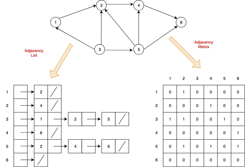
Graph Representations
The two most common ways to represent graphs in code are adjacency lists and adjacency matrices, each with its own strengths and weaknesses. When deciding on a graph implementation, it's important to understand the type of data and operations you will be using.

Adjacency List
In an adjacency list, the graph stores a list of vertices and for each vertex, a list of each vertex to which it's connected. So, for the following graph…
…an adjacency list in Python could look something like this:
    class Graph:
        def __init__(self):
            self.vertices = {
                              "A": {"B"},
                              "B": {"C", "D"},
                              "C": {"E"},
                              "D": {"F", "G"},
                              "E": {"C"},
                              "F": {"C"},
                              "G": {"A", "F"}
                            }
Note that this adjacency list doesn't actually use any lists. The vertices collection is a dictionary which lets us access each collection of edges in O(1) constant time while the edges are contained in a set which lets us check for the existence of edges in O(1) constant time.
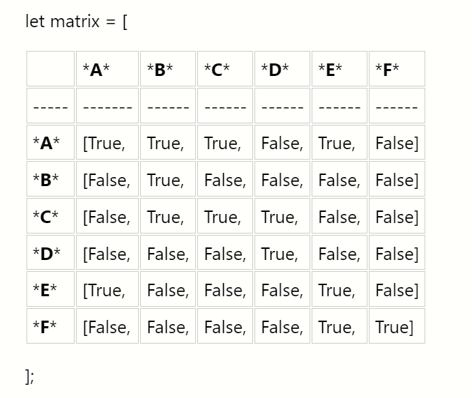
Adjacency Matrix
Now, let's see what this graph might look like as an adjacency matrix:
    class Graph:
        def __init__(self):
            self.edges = [[0,1,0,0,0,0,0],
                          [0,0,1,1,0,0,0],
                          [0,0,0,0,1,0,0],
                          [0,0,0,0,0,1,1],
                          [0,0,1,0,0,0,0],
                          [0,0,1,0,0,0,0],
                          [1,0,0,0,0,1,0]]
We represent this matrix as a two-dimensional array, or a list of lists. With this implementation, we get the benefit of built-in edge weights but do not have an association between the values of our vertices and their index.
In practice, both of these would probably contain more information by including Vertex or Edge classes.
Tradeoffs
Both adjacency matrices and adjacency lists have their own strengths and weaknesses. Let's explore their tradeoffs.
For the following:
V: Total number of vertices in the graph
E: Total number of edges in the graph
e: Average number of edges per vertex
Space Complexity
- Adjacency Matrix: O(V ^ 2)
- Adjacency List: O(V + E)
Consider a sparse graph with 100 vertices and only one edge. An adjacency list would have to store all 100 vertices but only needs to keep track of that single edge. The adjacency matrix would need to store 100x100=10,000 possible connections, even though all but one would be 0.
Now consider a dense graph where each vertex points to each other vertex. In this case, the total number of edges will approach V2 so the space complexities of each are comparable. However, dictionaries and sets are less space efficient than lists so for dense graphs, the adjacency matrix is more efficient.
Takeaway: Adjacency lists are more space efficient for sparse graphs while adjacency matrices become efficient for dense graphs.
Add Vertex
- Adjacency Matrix: O(V)
- Adjacency List: O(1)
Adding a vertex is extremely simple in an adjacency list:
self.vertices["H"] = set()
Adding a new key to a dictionary is a constant-time operation.
For an adjacency matrix, we would need to add a new value to the end of each existing row, then add a new row at the end.
for v in self.edges:
  self.edges[v].append(0)
v.append([0] * len(self.edges + 1))
Remember that with Python lists, appending to the end of a list is usually O(1) due to over-allocation of memory but can be O(n) when the over-allocated memory fills up. When this occurs, adding the vertex can be O(V2).
Takeaway: Adding vertices is very efficient in adjacency lists but very inefficient for adjacency matrices.
Remove Vertex
- Adjacency Matrix: O(V ^ 2)
- Adjacency List: O(V)
Removing vertices is pretty inefficient in both representations. In an adjacency matrix, we need to remove the removed vertex's row, then remove that column from each other row. Removing an element from a list requires moving everything after that element over by one slot which takes an average of V/2 operations. Since we need to do that for every single row in our matrix, that results in a V2 time complexity. On top of that, we need to reduce the index of each vertex after our removed index by 1 as well which doesn't add to our quadratic time complexity, but does add extra operations.
For an adjacency list, we need to visit each vertex and remove all edges pointing to our removed vertex. Removing elements from sets and dictionaries is a O(1) operation, so this results in an overall O(V) time complexity.
Takeaway: Removing vertices is inefficient in both adjacency matrices and lists but more inefficient in matrices.
Add Edge
- Adjacency Matrix: O(1)
- Adjacency List: O(1)
Adding an edge in an adjacency matrix is quite simple:
self.edges[v1][v2] = 1
Adding an edge in an adjacency list is similarly simple:
self.vertices[v1].add(v2)
Both are constant-time operations.
Takeaway: Adding edges to both adjacency lists and matrices is very efficient.
Remove Edge
- Adjacency Matrix: O(1)
- Adjacency List: O(1)
Removing an edge from an adjacency matrix is quite simple:
self.edges[v1][v2] = 0
Removing an edge from an adjacency list is similarly simple:
self.vertices[v1].remove(v2)
Both are constant-time operations.
Takeaway: Removing edges from both adjacency lists and matrices is very efficient.
Find Edge
- Adjacency Matrix: O(1)
- Adjacency List: O(1)
Finding an edge in an adjacency matrix is quite simple:
return self.edges[v1][v2] > 0
Finding an edge in an adjacency list is similarly simple:
return v2 in self.vertices[v1]
Both are constant-time operations.
Takeaway: Finding edges from both adjacency lists and matrices is very efficient.
Get All Edges from Vertex
- Adjacency Matrix: O(V)
- Adjacency List: O(1)
Say you want to know all the edges originating from a particular vertex. With an adjacency list, this is as simple as returning the value from the vertex dictionary:
return self.vertex[v]
In an adjacency matrix, however, it's a bit more complicated. You would need to iterate through the entire row and populate a list based on the results:
v_edges = []
for v2 in self.edges[v]:
    if self.edges[v][v2] > 0:
        v_edges.append(v2)
return v_edges
Takeaway: Fetching all edges is more efficient in an adjacency list than an adjacency matrix.
Breadth-First Search
Can use breadth-first search when searching a graph; explores graph outward in rings of increasing distance from starting vertex; never attempts to explore vertex it is or has already explored
BFS

Applications of BFS
- pathfinding, routing
- web crawlers
- find neighbor nodes in P2P network
- finding people/connections away on social network
- find neighboring locations on graph
- broadcasting on a network
- cycle detection in a graph
- finding connected components
- solving several theoretical graph problems
Coloring BFS
It's useful to color vertexes as you arrive at them and as you leave them behind as already searched.
unlisted: white
vertices whose neighbors are being explored: gray
vertices with no unexplored neighbors: black
BFS Pseudocode
    def BFS(graph, start_vert):
        for v of graph.vertices:
            v.color = white
        start_vert.color = gray
        queue.enqueue(start_vert)
        while !queue isEmpty():
        # peek at head but don't dequeue
        u = queue[0]
        for v of u.neighbors:
            if v.color == white:
                v.color == gray
                queue.enqueue(v)
        queue.dequeue()
        u.color = black
BFS Steps
- Mark graph vertices white.
- Mark starting vertex gray.
- Enqueue starting vertex.
- Check if queue is not empty.
- If not empty, peek at first item in queue.
- Loop through that vertex's neighbors.
- Check if unvisited.
- If unvisited, mark as gray and enqueue vertex.
- Dequeue current vertex and mark as black.
- Repeat until all vertices are explored.
Depth-First Search
dives down the graph as far as it can before backtracking and exploring another branch; never attempts to explore a vertex it has already explored or is in the process of exploring; exact order will vary depending on which branches get taken first and which is starting vertex
DFS
Applications of DFS
- preferred method for exploring a graph if we want to ensure we visit every node in graph
- finding minimum spanning trees of weighted graphs
- pathfinding
- detecting cycles in graphs
- solving and generating mazes
- topological sorting, useful for scheduling sequences of dependent jobs
DFS Pseudocode
    # recursion
    def explore(graph):
        visit(this_vert)
        explore(remaining_graph)

    # iterative
    def DFS(graph):
        for v of graph.verts:
            v.color = white
            v.parent = null
        for v of graph.verts:
            if v.color == white:
                DFS_visit(v)

    def DFS_visit(v):
        v.color = gray
        for neighbor of v.adjacent_nodes:
            if neighbor.color == white:
                neighbor.parent = v
                DFS_visit(neighbor)
        v.color = black
DFS Steps
- Take graph as parameter.
- Marks all vertices as unvisited.
- Sets vertex parent as null.
- Passes each unvisited vertex into DFS_visit().
- Mark current vertex as gray.
- Loops through its unvisited neighbors.
- Sets parent and makes recursive call to DFS_visit().
- Marks vertex as black.
- Repeat until done.
Connected Components
connected components: in a disjoint graph, groups of nodes on a graph that are connected with each other
Uses
- typically very large graphs, networks
- social networks
- networks (which devices can reach one another)
- epidemics (how spread, who started, where next)
key to finding connected components: searching algorithms, breadth-first search
How to find connected componnents
- for each node in graph:
- has it been explored
- if no, do BFS
- all nodes reached are connected
- if yes, already in connected component
- go to next node
strongly connected components: any node in this group can get to any other node
Bonus Python Question
'''py
This Bellman-Ford Code is for determination whether we can get
shortest path from given graph or not for single-source shortest-paths problem.
In other words, if given graph has any negative-weight cycle that is reachable
from the source, then it will give answer False for "no solution exits".
For argument graph, it should be a dictionary type
such as
graph = {

'a': {'b': 6, 'e': 7},

'b': {'c': 5, 'd': -4, 'e': 8},

'c': {'b': -2},

'd': {'a': 2, 'c': 7},

'e': {'b': -3}

}
Review of Concepts
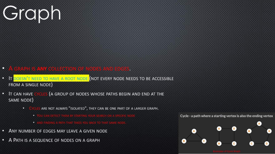
- A graph is any collection of nodes and edges.
- A graph is a less restrictive class of collections of nodes than structures like a tree.
- It doesn't need to have a root node (not every node needs to be accessible from a single node)
- It can have cycles (a group of nodes whose paths begin and end at the same node)
 - Any number of edges may leave a given node
- A Path is a sequence of nodes on a graph
### Undirected Graph
**Undirected Graph:** An undirected graph is one where the edges do not specify a particular direction. The edges are bi-directional.
### Types
- Any number of edges may leave a given node
- A Path is a sequence of nodes on a graph
### Undirected Graph
**Undirected Graph:** An undirected graph is one where the edges do not specify a particular direction. The edges are bi-directional.
### Types
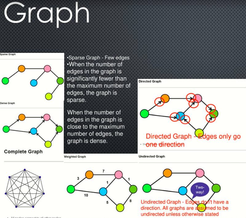
Dense Graph
- Dense Graph — A graph with lots of edges.
- "Dense graphs have many edges. But, wait! 🚧 I know what you must be thinking, how can you determine what qualifies as "many edges"? This is a little bit too subjective, right? ? I agree with you, so let's quantify it a little bit:
- Let's find the maximum number of edges in a directed graph. If there are |V| nodes in a directed graph (in the example below, six nodes), that means that each node can have up to |v| connections (in the example below, six connections).
- Why? Because each node could potentially connect with all other nodes and with itself (see "loop" below). Therefore, the maximum number of edges that the graph can have is |V|\*|V| , which is the total number of nodes multiplied by the maximum number of connections that each node can have."
- When the number of edges in the graph is close to the maximum number of edges, the graph is dense.
Sparse Graph
- Sparse Graph — Few edges
- When the number of edges in the graph is significantly fewer than the maximum number of edges, the graph is sparse.
Weighted Graph
- Weighted Graph — Edges have a cost or a weight to traversal
Directed Graph
- Directed Graph — Edges only go one direction
Undirected Graph
- Undirected Graph — Edges don't have a direction. All graphs are assumed to be undirected unless otherwise stated
Node Class
Uses a class to define the neighbors as properties of each node.
Adjacency Matrix
The row index will correspond to the source of an edge and the column index will correspond to the edges destination.
- When the edges have a direction,
matrix[i][j]may not be the same asmatrix[j][i] - It is common to say that a node is adjacent to itself so
matrix[x][x]is true for any node - Will be O(n2) space complexity
Adjacency List
Seeks to solve the shortcomings of the matrix implementation. It uses an object where keys represent node labels and values associated with that key are the adjacent node keys held in an array.
Stacks
- The Call Stack is a Stack data structure, and is used to manage the order of function invocations in your code.
- Browser History is often implemented using a Stack, with one great example being the browser history object in the very popular React Router module.
- Undo/Redo functionality in just about any application. For example:
- When you're coding in your text editor, each of the actions you take on your keyboard are recorded by
pushing that event to a Stack. - When you hit [cmd + z] to undo your most recent action, that event is
poped off the Stack, because the last event that occured should be the first one to be undone (LIFO). - When you hit [cmd + y] to redo your most recent action, that event is
pushed back onto the Stack.
Queues
- Printers use a Queue to manage incoming jobs to ensure that documents are printed in the order they are received.
- Chat rooms, online video games, and customer service phone lines use a Queue to ensure that patrons are served in the order they arrive.
- In the case of a Chat Room, to be admitted to a size-limited room.
- In the case of an Online Multi-Player Game, players wait in a lobby until there is enough space and it is their turn to be admitted to a game.
- In the case of a Customer Service Phone Line…you get the point.
- As a more advanced use case, Queues are often used as components or services in the system design of a service-oriented architecture. A very popular and easy to use example of this is Amazon's Simple Queue Service (SQS), which is a part of their Amazon Web Services (AWS) offering.
- You would add this service to your system between two other services, one that is sending information for processing, and one that is receiving information to be processed, when the volume of incoming requests is high and the integrity of the order with which those requests are processed must be maintained.
Further resources:
bgoonz's gists
Instantly share code, notes, and snippets. Web Developer, Electrical Engineer JavaScript | CSS | Bootstrap | Python |…gist.github.com
Data Structures Reference
Data Structures… Under The Hood
Data Structures Reference
Array
Stores things in order. Has quick lookups by index.
Linked List
Also stores things in order. Faster insertions and deletions than
arrays, but slower lookups (you have to "walk down" the whole list).
!
Queue
Like the line outside a busy restaurant. "First come, first served."
Stack
Like a stack of dirty plates in the sink. The first one you take off the
top is the last one you put down.
Tree
Good for storing hierarchies. Each node can have "child" nodes.
Binary Search Tree
Everything in the left subtree is smaller than the current node,
everything in the right subtree is larger. lookups, but only if the tree
is balanced!
Binary Search Tree
Graph
Good for storing networks, geography, social relationships, etc.
Heap
A binary tree where the smallest value is always at the top. Use it to implement a priority queue.
![A binary heap is a binary tree where the nodes are organized to so that the smallest value is always at the top.]
Adjacency list
A list where the index represents the node and the value at that index is a list of the node's neighbors:
graph = [ [1], [0, 2, 3], [1, 3], [1, 2], ]
Since node 3 has edges to nodes 1 and 2, graph[3] has the adjacency list [1, 2].
We could also use a dictionary where the keys represent the node and the values are the lists of neighbors.
graph = { 0: [1], 1: [0, 2, 3], 2: [1, 3], 3: [1, 2], }
This would be useful if the nodes were represented by strings, objects, or otherwise didn't map cleanly to list indices.
Adjacency matrix
A matrix of 0s and 1s indicating whether node x connects to node y (0 means no, 1 means yes).
graph = [ [0, 1, 0, 0], [1, 0, 1, 1], [0, 1, 0, 1], [0, 1, 1, 0], ]
Since node 3 has edges to nodes 1 and 2, graph[3][1] and graph[3][2] have value 1.
a = LinkedListNode(5) b = LinkedListNode(1) c = LinkedListNode(9) a.next = b b.next = c
Arrays
Ok, so we know how to store individual numbers. Let's talk about storing several numbers.
That's right, things are starting to heat up.
Suppose we wanted to keep a count of how many bottles of kombucha we drink every day.
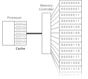
Let's store each day's kombucha count in an 8-bit, fixed-width, unsigned integer. That should be plenty — we're not likely to get through more than 256 (28) bottles in a single day, right?
And let's store the kombucha counts right next to each other in RAM, starting at memory address 0:
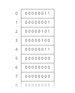 Bam. That's an **array**. RAM is*basically* an array already.
Just like with RAM, the elements of an array are numbered. We call that number the **index** of the array element (plural: indices). In _this_ example, each array element's index is the same as its address in RAM.
But that's not usually true. Suppose another program like Spotify had already stored some information at memory address 2:
Bam. That's an **array**. RAM is*basically* an array already.
Just like with RAM, the elements of an array are numbered. We call that number the **index** of the array element (plural: indices). In _this_ example, each array element's index is the same as its address in RAM.
But that's not usually true. Suppose another program like Spotify had already stored some information at memory address 2:
 We'd have to start our array below it, for example at memory address 3. So index 0 in our array would be at memory address 3, and index 1 would be at memory address 4, etc.:
 Suppose we wanted to get the kombucha count at index 4 in our array. How do we figure out what*address in memory* to go to? Simple math:
Take the array's starting address (3), add the index we're looking for (4), and that's the address of the item we're looking for. 3 + 4 = 7. In general, for getting the nth item in our array:
\\text{address of nth item in array} = \\text{address of array start} + n
This works out nicely because the size of the addressed memory slots and the size of each kombucha count are _both_ 1 byte. So a slot in our array corresponds to a slot in RAM.
But that's not always the case. In fact, it's _usually not_ the case. We _usually_ use _64-bit_ integers.
So how do we build an array of _64-bit_ (8 byte) integers on top of our _8-bit_ (1 byte) memory slots?
We simply give each array index _8_ address slots instead of 1:
Suppose we wanted to get the kombucha count at index 4 in our array. How do we figure out what*address in memory* to go to? Simple math:
Take the array's starting address (3), add the index we're looking for (4), and that's the address of the item we're looking for. 3 + 4 = 7. In general, for getting the nth item in our array:
\\text{address of nth item in array} = \\text{address of array start} + n
This works out nicely because the size of the addressed memory slots and the size of each kombucha count are _both_ 1 byte. So a slot in our array corresponds to a slot in RAM.
But that's not always the case. In fact, it's _usually not_ the case. We _usually_ use _64-bit_ integers.
So how do we build an array of _64-bit_ (8 byte) integers on top of our _8-bit_ (1 byte) memory slots?
We simply give each array index _8_ address slots instead of 1:
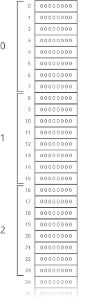 So we can still use simple math to grab the start of the nth item in our array — just gotta throw in some multiplication:
\\text{address of nth item in array} = \\text{address of array start} + (n \* \\text{size of each item in bytes})
Don't worry — adding this multiplication doesn't really slow us down. Remember: addition, subtraction, multiplication, and division of fixed-width integers takes time. So _all_ the math we're using here to get the address of the nth item in the array takes time.
And remember how we said the memory controller has a _direct connection_ to each slot in RAM? That means we can read the stuff at any given memory address in time.
So we can still use simple math to grab the start of the nth item in our array — just gotta throw in some multiplication:
\\text{address of nth item in array} = \\text{address of array start} + (n \* \\text{size of each item in bytes})
Don't worry — adding this multiplication doesn't really slow us down. Remember: addition, subtraction, multiplication, and division of fixed-width integers takes time. So _all_ the math we're using here to get the address of the nth item in the array takes time.
And remember how we said the memory controller has a _direct connection_ to each slot in RAM? That means we can read the stuff at any given memory address in time.
 **Together, this means looking up the contents of a given array index is time.** This fast lookup capability is the most important property of arrays.
But the formula we used to get the address of the nth item in our array only works _if_:
1. **Each item in the array is the _same size_** (takes up the same
number of bytes).
1. **The array is _uninterrupted_ (contiguous) in memory**. There can't
be any gaps in the array…like to "skip over" a memory slot Spotify was already using.
These things make our formula for finding the nth item _work_ because they make our array _predictable_. We can _predict_ exactly where in memory the nth element of our array will be.
But they also constrain what kinds of things we can put in an array. Every item has to be the same size. And if our array is going to store a _lot_ of stuff, we'll need a _bunch_ of uninterrupted free space in RAM. Which gets hard when most of our RAM is already occupied by other programs (like Spotify).
That's the tradeoff. Arrays have fast lookups ( time), but each item in the array needs to be the same size, and you need a big block of uninterrupted free memory to store the array.
--------
## Pointers
Remember how we said every item in an array had to be the same size? Let's dig into that a little more.
Suppose we wanted to store a bunch of ideas for baby names. Because we've got some _really_ cute ones.
Each name is a string. Which is really an array. And now we want to store _those arrays_ in an array. _Whoa_.
Now, what if our baby names have different lengths? That'd violate our rule that all the items in an array need to be the same size!
We could put our baby names in arbitrarily large arrays (say, 13 characters each), and just use a special character to mark the end of the string within each array…
**Together, this means looking up the contents of a given array index is time.** This fast lookup capability is the most important property of arrays.
But the formula we used to get the address of the nth item in our array only works _if_:
1. **Each item in the array is the _same size_** (takes up the same
number of bytes).
1. **The array is _uninterrupted_ (contiguous) in memory**. There can't
be any gaps in the array…like to "skip over" a memory slot Spotify was already using.
These things make our formula for finding the nth item _work_ because they make our array _predictable_. We can _predict_ exactly where in memory the nth element of our array will be.
But they also constrain what kinds of things we can put in an array. Every item has to be the same size. And if our array is going to store a _lot_ of stuff, we'll need a _bunch_ of uninterrupted free space in RAM. Which gets hard when most of our RAM is already occupied by other programs (like Spotify).
That's the tradeoff. Arrays have fast lookups ( time), but each item in the array needs to be the same size, and you need a big block of uninterrupted free memory to store the array.
--------
## Pointers
Remember how we said every item in an array had to be the same size? Let's dig into that a little more.
Suppose we wanted to store a bunch of ideas for baby names. Because we've got some _really_ cute ones.
Each name is a string. Which is really an array. And now we want to store _those arrays_ in an array. _Whoa_.
Now, what if our baby names have different lengths? That'd violate our rule that all the items in an array need to be the same size!
We could put our baby names in arbitrarily large arrays (say, 13 characters each), and just use a special character to mark the end of the string within each array…
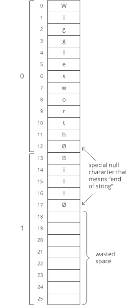 "Wigglesworth" is a cute baby name, right?
But look at all that wasted space after "Bill". And what if we wanted to store a string that was _more_ than 13 characters? We'd be out of luck.
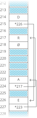
There's a better way. Instead of storing the strings right inside our array, let's just put the strings wherever we can fit them in memory. Then we'll have each element in our array hold the _address in memory_ of its corresponding string. Each address is an integer, so really our outer array is just an array of integers. We can call each of these integers a **pointer**, since it points to another spot in memory.
"Wigglesworth" is a cute baby name, right?
But look at all that wasted space after "Bill". And what if we wanted to store a string that was _more_ than 13 characters? We'd be out of luck.
There's a better way. Instead of storing the strings right inside our array, let's just put the strings wherever we can fit them in memory. Then we'll have each element in our array hold the _address in memory_ of its corresponding string. Each address is an integer, so really our outer array is just an array of integers. We can call each of these integers a **pointer**, since it points to another spot in memory.
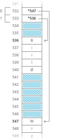 The pointers are marked with a \* at the beginning.
Pretty clever, right? This fixes _both_ the disadvantages of arrays:
1. The items don't have to be the same length — each string can be as
long or as short as we want.
1. We don't need enough uninterrupted free memory to store all our
strings next to each other — we can place each of them separately, wherever there's space in RAM.
We fixed it! No more tradeoffs. Right?
Nope. Now we have a _new_ tradeoff:
Remember how the memory controller sends the contents of _nearby_ memory addresses to the processor with each read? And the processor caches them? So reading sequential addresses in RAM is _faster_ because we can get most of those reads right from the cache?
The pointers are marked with a \* at the beginning.
Pretty clever, right? This fixes _both_ the disadvantages of arrays:
1. The items don't have to be the same length — each string can be as
long or as short as we want.
1. We don't need enough uninterrupted free memory to store all our
strings next to each other — we can place each of them separately, wherever there's space in RAM.
We fixed it! No more tradeoffs. Right?
Nope. Now we have a _new_ tradeoff:
Remember how the memory controller sends the contents of _nearby_ memory addresses to the processor with each read? And the processor caches them? So reading sequential addresses in RAM is _faster_ because we can get most of those reads right from the cache?
 Our original array was very **cache-friendly**, because everything was sequential. So reading from the 0th index, then the 1st index, then the 2nd, etc. got an extra speedup from the processor cache.
**But the pointers in this array make it _not_ cache-friendly**, because the baby names are scattered randomly around RAM. So reading from the 0th index, then the 1st index, etc. doesn't get that extra speedup from the cache.
That's the tradeoff. This pointer-based array requires less uninterrupted memory and can accommodate elements that aren't all the same size, _but_ it's _slower_ because it's not cache-friendly.
This slowdown isn't reflected in the big O time cost. Lookups in this pointer-based array are _still_ time.
--------
### Linked lists
Our word processor is definitely going to need fast appends — appending to the document is like the _main thing_ you do with a word processor.
Can we build a data structure that can store a string, has fast appends, _and_ doesn't require you to say how long the string will be ahead of time?
Let's focus first on not having to know the length of our string ahead of time. Remember how we used _pointers_ to get around length issues with our array of baby names?
What if we pushed that idea even further?
What if each _character_ in our string were a _two-index array_ with:
1. the character itself 2. a pointer to the next character
Our original array was very **cache-friendly**, because everything was sequential. So reading from the 0th index, then the 1st index, then the 2nd, etc. got an extra speedup from the processor cache.
**But the pointers in this array make it _not_ cache-friendly**, because the baby names are scattered randomly around RAM. So reading from the 0th index, then the 1st index, etc. doesn't get that extra speedup from the cache.
That's the tradeoff. This pointer-based array requires less uninterrupted memory and can accommodate elements that aren't all the same size, _but_ it's _slower_ because it's not cache-friendly.
This slowdown isn't reflected in the big O time cost. Lookups in this pointer-based array are _still_ time.
--------
### Linked lists
Our word processor is definitely going to need fast appends — appending to the document is like the _main thing_ you do with a word processor.
Can we build a data structure that can store a string, has fast appends, _and_ doesn't require you to say how long the string will be ahead of time?
Let's focus first on not having to know the length of our string ahead of time. Remember how we used _pointers_ to get around length issues with our array of baby names?
What if we pushed that idea even further?
What if each _character_ in our string were a _two-index array_ with:
1. the character itself 2. a pointer to the next character
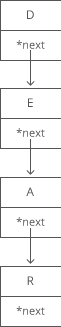 We would call each of these two-item arrays a **node** and we'd call this series of nodes a **linked list**.
Here's how we'd actually implement it in memory:
We would call each of these two-item arrays a **node** and we'd call this series of nodes a **linked list**.
Here's how we'd actually implement it in memory:
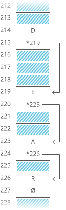 Notice how we're free to store our nodes wherever we can find two open slots in memory. They don't have to be next to each other. They don't even have to be*in order*:
 "But that's not cache-friendly, " you may be thinking. Good point! We'll get to that.
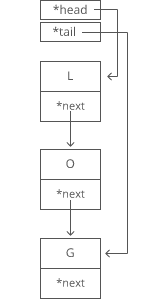
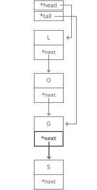
The first node of a linked list is called the **head**, and the last node is usually called the **tail**.
Confusingly, some people prefer to use "tail" to refer to _everything after the head_ of a linked list. In an interview it's fine to use either definition. Briefly say which definition you're using, just to be clear.
It's important to have a pointer variable referencing the head of the list — otherwise we'd be unable to find our way back to the start of the list!
We'll also sometimes keep a pointer to the tail. That comes in handy when we want to add something new to the end of the linked list. In fact, let's try that out:
Suppose we had the string "LOG" stored in a linked list:
"But that's not cache-friendly, " you may be thinking. Good point! We'll get to that.
The first node of a linked list is called the **head**, and the last node is usually called the **tail**.
Confusingly, some people prefer to use "tail" to refer to _everything after the head_ of a linked list. In an interview it's fine to use either definition. Briefly say which definition you're using, just to be clear.
It's important to have a pointer variable referencing the head of the list — otherwise we'd be unable to find our way back to the start of the list!
We'll also sometimes keep a pointer to the tail. That comes in handy when we want to add something new to the end of the linked list. In fact, let's try that out:
Suppose we had the string "LOG" stored in a linked list:
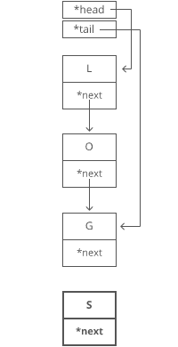
 Suppose we wanted to add an "S" to the end, to make it "LOGS". How would we do that?
Easy. We just put it in a new node:
Suppose we wanted to add an "S" to the end, to make it "LOGS". How would we do that?
Easy. We just put it in a new node:
 And tweak some pointers:
1. Grab the last letter, which is "G". Our tail pointer lets us do this in time.
And tweak some pointers:
1. Grab the last letter, which is "G". Our tail pointer lets us do this in time.
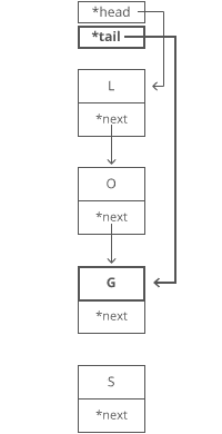 2. Point the last letter's next to the letter we're appending ("S").
 3. Update the tail pointer to point to our*new* last letter, "S".
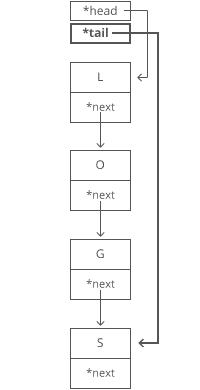 That's time.
Why is it time? Because the runtime doesn't get bigger if the string gets bigger. No matter how many characters are in our string, we still just have to tweak a couple pointers for any append.
Now, what if instead of a linked list, our string had been a _dynamic array_? We might not have any room at the end, forcing us to do one of those doubling operations to make space:
That's time.
Why is it time? Because the runtime doesn't get bigger if the string gets bigger. No matter how many characters are in our string, we still just have to tweak a couple pointers for any append.
Now, what if instead of a linked list, our string had been a _dynamic array_? We might not have any room at the end, forcing us to do one of those doubling operations to make space:
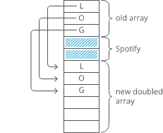 So with a dynamic array, our append would have a*worst-case* time cost of .
**Linked lists have worst-case -time appends, which is better than the worst-case time of dynamic arrays.**
That _worst-case_ part is important. The _average case_ runtime for appends to linked lists and dynamic arrays is the same: .
Now, what if we wanted to \*pre\*pend something to our string? Let's say we wanted to put a "B" at the beginning.
For our linked list, it's just as easy as appending. Create the node:
So with a dynamic array, our append would have a*worst-case* time cost of .
**Linked lists have worst-case -time appends, which is better than the worst-case time of dynamic arrays.**
That _worst-case_ part is important. The _average case_ runtime for appends to linked lists and dynamic arrays is the same: .
Now, what if we wanted to \*pre\*pend something to our string? Let's say we wanted to put a "B" at the beginning.
For our linked list, it's just as easy as appending. Create the node:
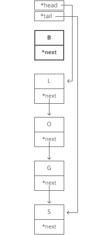 And tweak some pointers:
1. Point "B"'s next to "L". 2. Point the head to "B".
And tweak some pointers:
1. Point "B"'s next to "L". 2. Point the head to "B".
 Bam. time again.
But if our string were a _dynamic array_…
Bam. time again.
But if our string were a _dynamic array_…
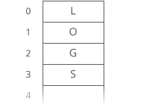 And we wanted to add in that "B":
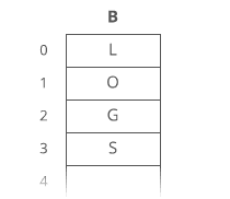 Eep. We have to*make room* for the "B"!
We have to move _each character_ one space down:
Eep. We have to*make room* for the "B"!
We have to move _each character_ one space down:
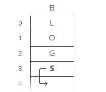

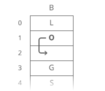
 *Now* we can drop the "B" in there:
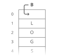 What's our time cost here?
It's all in the step where we made room for the first letter. We had to move _all n_ characters in our string. One at a time. That's time.
**So linked lists have faster \*pre\*pends ( time) than dynamic arrays ( time).**
No "worst case" caveat this time — prepends for dynamic arrays are _always_ time. And prepends for linked lists are _always_ time.
These quick appends and prepends for linked lists come from the fact that linked list nodes can go anywhere in memory. They don't have to sit right next to each other the way items in an array do.
So if linked lists are so great, why do we usually store strings in an array? **Because**
arrays have -time lookups
**.** And those constant-time lookups _come from_ the fact that all the array elements are lined up next to each other in memory.
Lookups with a linked list are more of a process, because we have no way of knowing where the ith node is in memory. So we have to walk through the linked list node by node, counting as we go, until we hit the ith item.
def get_ith_item_in_linked_list(head, i): if i < 0: raise ValueError("i can't be negative: %d" % i) current_node = head current_position = 0 while current_node: if current_position == i: \# Found it! return current_node \# Move on to the next node current_node = current_node.next current_position += 1 raise ValueError('List has fewer than i + 1 (%d) nodes' % (i + 1))
That's i + 1 steps down our linked list to get to the ith node (we made our function zero-based to match indices in arrays). **So linked lists have -time lookups.** Much slower than the -time lookups for arrays and dynamic arrays.
Not only that — **walking down a linked list is _not_ cache-friendly.** Because the next node could be _anywhere_ in memory, we don't get any benefit from the processor cache. This means lookups in a linked list are even slower.
So the tradeoff with linked lists is they have faster prepends and faster appends than dynamic arrays, _but_ they have slower lookups.
--------
## Doubly Linked Lists
In a basic linked list, each item stores a single pointer to the next element.
In a **doubly linked list**, items have pointers to the next _and the previous_ nodes.
What's our time cost here?
It's all in the step where we made room for the first letter. We had to move _all n_ characters in our string. One at a time. That's time.
**So linked lists have faster \*pre\*pends ( time) than dynamic arrays ( time).**
No "worst case" caveat this time — prepends for dynamic arrays are _always_ time. And prepends for linked lists are _always_ time.
These quick appends and prepends for linked lists come from the fact that linked list nodes can go anywhere in memory. They don't have to sit right next to each other the way items in an array do.
So if linked lists are so great, why do we usually store strings in an array? **Because**
arrays have -time lookups
**.** And those constant-time lookups _come from_ the fact that all the array elements are lined up next to each other in memory.
Lookups with a linked list are more of a process, because we have no way of knowing where the ith node is in memory. So we have to walk through the linked list node by node, counting as we go, until we hit the ith item.
def get_ith_item_in_linked_list(head, i): if i < 0: raise ValueError("i can't be negative: %d" % i) current_node = head current_position = 0 while current_node: if current_position == i: \# Found it! return current_node \# Move on to the next node current_node = current_node.next current_position += 1 raise ValueError('List has fewer than i + 1 (%d) nodes' % (i + 1))
That's i + 1 steps down our linked list to get to the ith node (we made our function zero-based to match indices in arrays). **So linked lists have -time lookups.** Much slower than the -time lookups for arrays and dynamic arrays.
Not only that — **walking down a linked list is _not_ cache-friendly.** Because the next node could be _anywhere_ in memory, we don't get any benefit from the processor cache. This means lookups in a linked list are even slower.
So the tradeoff with linked lists is they have faster prepends and faster appends than dynamic arrays, _but_ they have slower lookups.
--------
## Doubly Linked Lists
In a basic linked list, each item stores a single pointer to the next element.
In a **doubly linked list**, items have pointers to the next _and the previous_ nodes.
 Doubly linked lists allow us to traverse our list*backwards*. In a*singly*linked list, if you just had a pointer to a node in the*middle*of a list, there would be*no way* to know what nodes came before it. Not a problem in a doubly linked list.
### Not cache-friendly
Most computers have caching systems that make reading from sequential addresses in memory faster than reading from scattered addresses.
Array items are always located right next to each other in computer memory, but linked list nodes can be scattered all over.
So iterating through a linked list is usually quite a bit slower than iterating through the items in an array, even though they're both theoretically time.
--------
### Hash tables
Quick lookups are often really important. For that reason, we tend to use arrays (-time lookups) much more often than linked lists (-time lookups).
For example, suppose we wanted to count how many times each ASCII character appears in Romeo and Juliet. How would we store those counts?
We can use arrays in a clever way here. Remember — characters are just numbers. In ASCII (a common character encoding) 'A' is 65, 'B' is 66, etc.
So we can use the character('s number value) as the _index_ in our array, and store the _count_ for that character _at that index_ in the array:
Doubly linked lists allow us to traverse our list*backwards*. In a*singly*linked list, if you just had a pointer to a node in the*middle*of a list, there would be*no way* to know what nodes came before it. Not a problem in a doubly linked list.
### Not cache-friendly
Most computers have caching systems that make reading from sequential addresses in memory faster than reading from scattered addresses.
Array items are always located right next to each other in computer memory, but linked list nodes can be scattered all over.
So iterating through a linked list is usually quite a bit slower than iterating through the items in an array, even though they're both theoretically time.
--------
### Hash tables
Quick lookups are often really important. For that reason, we tend to use arrays (-time lookups) much more often than linked lists (-time lookups).
For example, suppose we wanted to count how many times each ASCII character appears in Romeo and Juliet. How would we store those counts?
We can use arrays in a clever way here. Remember — characters are just numbers. In ASCII (a common character encoding) 'A' is 65, 'B' is 66, etc.
So we can use the character('s number value) as the _index_ in our array, and store the _count_ for that character _at that index_ in the array:
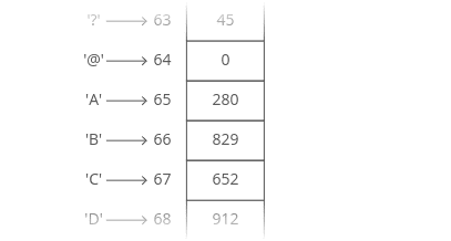 With this array, we can look up (and edit) the count for any character in constant time. Because we can access any index in our array in constant time.
Something interesting is happening here — this array isn't just a list of values. This array is storing _two_ things: characters and counts. The characters are _implied_ by the indices.
**So we can think of an array as a _table_ with _two columns_…except you don't really get to pick the values in one column (the indices) — they're always 0, 1, 2, 3, etc.**
But what if we wanted to put _any_ value in that column and still get quick lookups?
Suppose we wanted to count the number of times each _word_ appears in Romeo and Juliet. Can we adapt our array?
Translating a _character_ into an array index was easy. But we'll have to do something more clever to translate a _word_ (a string) into an array index…
With this array, we can look up (and edit) the count for any character in constant time. Because we can access any index in our array in constant time.
Something interesting is happening here — this array isn't just a list of values. This array is storing _two_ things: characters and counts. The characters are _implied_ by the indices.
**So we can think of an array as a _table_ with _two columns_…except you don't really get to pick the values in one column (the indices) — they're always 0, 1, 2, 3, etc.**
But what if we wanted to put _any_ value in that column and still get quick lookups?
Suppose we wanted to count the number of times each _word_ appears in Romeo and Juliet. Can we adapt our array?
Translating a _character_ into an array index was easy. But we'll have to do something more clever to translate a _word_ (a string) into an array index…
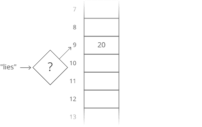 Here's one way we could do it:
Grab the number value for each character and add those up.
Here's one way we could do it:
Grab the number value for each character and add those up.
 The result is 429. But what if we only have*30* slots in our array? We'll use a common trick for forcing a number into a specific range: the modulus operator (%). Modding our sum by 30 ensures we get a whole number that's less than 30 (and at least 0):
429 \\: \\% \\: 30 = 9
Bam. That'll get us from a word (or any string) to an array index.
This data structure is called a **hash table** or **hash map**. In our hash table, the _counts_ are the **values** and the _words_ ("lies, " etc.) are the **keys** (analogous to the _indices_ in an array). The process we used to translate a key into an array index is called a **hashing function**.
!\[A blank array except for a 20, labeled as the value, stored at index
1. To the left the array is the word "lies," labeled as the key, with an
arrow pointing to the right at diamond with a question mark in the middle, labeled as the hashing function. The diamond points to the 9th index of the array.\](https://www.interviewcake.com/images/svgs/cs_for_hackers\_\_hash_tables_lies_key_labeled.svg?bust=209)
The hashing functions used in modern systems get pretty complicated — the one we used here is a simplified example.
Note that our quick lookups are only in one direction — we can quickly get the value for a given key, but the only way to get the key for a given value is to walk through all the values and keys.
Same thing with arrays — we can quickly look up the value at a given index, but the only way to figure out the index for a given value is to walk through the whole array.
One problem — what if two keys hash to the same index in our array? Look at "lies" and "foes":
The result is 429. But what if we only have*30* slots in our array? We'll use a common trick for forcing a number into a specific range: the modulus operator (%). Modding our sum by 30 ensures we get a whole number that's less than 30 (and at least 0):
429 \\: \\% \\: 30 = 9
Bam. That'll get us from a word (or any string) to an array index.
This data structure is called a **hash table** or **hash map**. In our hash table, the _counts_ are the **values** and the _words_ ("lies, " etc.) are the **keys** (analogous to the _indices_ in an array). The process we used to translate a key into an array index is called a **hashing function**.
!\[A blank array except for a 20, labeled as the value, stored at index
1. To the left the array is the word "lies," labeled as the key, with an
arrow pointing to the right at diamond with a question mark in the middle, labeled as the hashing function. The diamond points to the 9th index of the array.\](https://www.interviewcake.com/images/svgs/cs_for_hackers\_\_hash_tables_lies_key_labeled.svg?bust=209)
The hashing functions used in modern systems get pretty complicated — the one we used here is a simplified example.
Note that our quick lookups are only in one direction — we can quickly get the value for a given key, but the only way to get the key for a given value is to walk through all the values and keys.
Same thing with arrays — we can quickly look up the value at a given index, but the only way to figure out the index for a given value is to walk through the whole array.
One problem — what if two keys hash to the same index in our array? Look at "lies" and "foes":
 They both sum up to 429! So of course they'll have the same answer when we mod by 30:
429 \\: \\% \\: 30 = 9
So our hashing function gives us the same answer for "lies" and "foes." This is called a **hash collision**. There are a few different strategies for dealing with them.
Here's a common one: instead of storing the actual values in our array, let's have each array slot hold a _pointer_ to a _linked list_ holding the counts for all the words that hash to that index:
They both sum up to 429! So of course they'll have the same answer when we mod by 30:
429 \\: \\% \\: 30 = 9
So our hashing function gives us the same answer for "lies" and "foes." This is called a **hash collision**. There are a few different strategies for dealing with them.
Here's a common one: instead of storing the actual values in our array, let's have each array slot hold a _pointer_ to a _linked list_ holding the counts for all the words that hash to that index:
 One problem — how do we know which count is for "lies" and which is for "foes"? To fix this, we'll store the*word* as well as the count in each linked list node:
 "But wait!" you may be thinking, "Now lookups in our hash table take time in the worst case, since we have to walk down a linked list." That's true! You could even say that in the worst case*every*key creates a hash collision, so our whole hash table*degrades to a linked list*.
In industry though, we usually wave our hands and say **collisions are rare enough that on _average_ lookups in a hash table are time**. And there are fancy algorithms that keep the number of collisions low and keep the lengths of our linked lists nice and short.
But that's sort of the tradeoff with hash tables. You get fast lookups by key…except _some_ lookups could be slow. And of course, you only get those fast lookups in one direction — looking up the _key_ for a given _value_ still takes time
### Breadth-First Search (BFS) and Breadth-First Traversal
**Breadth-first search** (BFS) is a method for exploring a tree or graph. In a BFS, you first explore all the nodes one step away, then all the nodes two steps away, etc.
Breadth-first search is like throwing a stone in the center of a pond. The nodes you explore "ripple out" from the starting point.
Here's a how a BFS would traverse this tree, starting with the root:
"But wait!" you may be thinking, "Now lookups in our hash table take time in the worst case, since we have to walk down a linked list." That's true! You could even say that in the worst case*every*key creates a hash collision, so our whole hash table*degrades to a linked list*.
In industry though, we usually wave our hands and say **collisions are rare enough that on _average_ lookups in a hash table are time**. And there are fancy algorithms that keep the number of collisions low and keep the lengths of our linked lists nice and short.
But that's sort of the tradeoff with hash tables. You get fast lookups by key…except _some_ lookups could be slow. And of course, you only get those fast lookups in one direction — looking up the _key_ for a given _value_ still takes time
### Breadth-First Search (BFS) and Breadth-First Traversal
**Breadth-first search** (BFS) is a method for exploring a tree or graph. In a BFS, you first explore all the nodes one step away, then all the nodes two steps away, etc.
Breadth-first search is like throwing a stone in the center of a pond. The nodes you explore "ripple out" from the starting point.
Here's a how a BFS would traverse this tree, starting with the root:
 We'd visit all the immediate children (all the nodes that're one step away from our starting node):
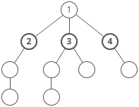 Then we'd move on to all*those*nodes' children (all the nodes that're*two steps* away from our starting node):
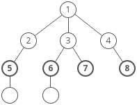 And so on:
 Until we reach the end.
Breadth-first search is often compared with **depth-first search**.
Advantages:
- A BFS will find the **shortest path** between the starting point and
any other reachable node. A depth-first search will not necessarily find the shortest path.
Disadvantages
- A BFS on a binary tree _generally_ requires more memory than a DFS.
Until we reach the end.
Breadth-first search is often compared with **depth-first search**.
Advantages:
- A BFS will find the **shortest path** between the starting point and
any other reachable node. A depth-first search will not necessarily find the shortest path.
Disadvantages
- A BFS on a binary tree _generally_ requires more memory than a DFS.
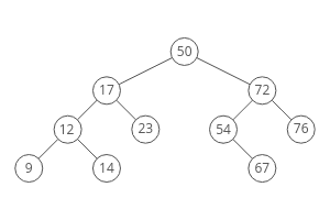
Binary Search Tree
A binary tree is a tree where <==(every node has two or fewer children)==>.
The children are usually called left and right.
class BinaryTreeNode(object):
This lets us build a structure like this:
That particular example is special because every level of the tree is completely full. There are no "gaps." We call this kind of tree "perfect."

Binary trees have a few interesting properties when they're perfect:
Property 1: the number of total nodes on each "level" doubles as we move down the tree.
Property 2: the number of nodes on the last level is equal to the sum of the number of nodes on all other levels (plus 1). In other words, about*half* of our nodes are on the last level.
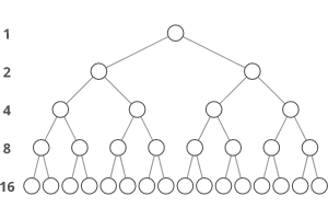
<==(**Let's call the number of nodes n, **)==>
<==(_and the height of the tree h. _)==>
h can also be thought of as the "number of levels."
If we had h, how could we calculate n?
Let's just add up the number of nodes on each level!
If we zero-index the levels, the number of nodes on the xth level is exactly 2^x.
- Level 0: 20 nodes,
- 2. Level 1: 21 nodes,
- 3. Level 2: 22 nodes,
- 4. Level 3: 23 nodes,
- 5. etc
So our total number of nodes is:
n = 20 + 21 + 22 + 23 + … + 2^{h-1}
Why only up to 2^{h-1}?
Notice that we started counting our levels at 0.
- So if we have h levels in total,
- the last level is actually the "h-1"-th level.
- That means the number of nodes on the last level is 2^{h-1}.
But we can simplify.
Property 2 tells us that the number of nodes on the last level is (1 more than) half of the total number of nodes,
so we can just take the number of nodes on the last level, multiply it by 2, and subtract 1 to get the number of nodes overall.
- We know the number of nodes on the last level is 2^{h-1},
- So:
n = 2^{h-1} * 2–1
n = 2^{h-1} * 21 — 1
n = 2^{h-1+1}- 1
n = 2^{h} — 1
So that's how we can go from h to n. What about the other direction?
We need to bring the h down from the exponent.
That's what logs are for!
First, some quick review.
<==(log_{10} (100) )==>
simply means,
"What power must you raise 10 to in order to get 100?".
Which is 2,
because .
<==(102 = 100 )==>
Graph Data Structure: Directed, Acyclic, etc
Graph =====
Binary numbers
Let's put those bits to use. Let's store some stuff. Starting with numbers.
The number system we usually use (the one you probably learned in elementary school) is called base 10, because each digit has ten possible values (1, 2, 3, 4, 5, 6, 7, 8, 9, and 0).
But computers don't have digits with ten possible values. They have bits with two possible values. So they use base 2 numbers.
Base 10 is also called decimal. Base 2 is also called binary.
To understand binary, let's take a closer look at how decimal numbers work. Take the number "101" in decimal:
Notice we have two "1"s here, but they don't*mean*the same thing. The leftmost "1"means*100, and the rightmost "1"*means 1. That's because the leftmost "1" is in the hundreds place, while the rightmost "1" is in the ones place. And the "0" between them is in the tens place.

So this "101" in base 10 is telling us we have "1 hundred, 0 tens, and 1 one."

Notice how the*places*in base 10 (ones place, tens place, hundreds place, etc.) are*sequential powers of 10*:
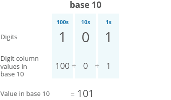
- 100=1 * 101=10 * 102=100 * 103=1000 * etc.
The places in binary (base 2) are sequential powers of 2:
- 20=1 * 21=2 * 22=4 * 23=8 * etc.
So let's take that same "101" but this time let's read it as a binary number:
Reading this from right to left: we have a 1 in the ones place, a 0 in the twos place, and a 1 in the fours place. So our total is 4 + 0 + 1 which is 5.

Implementations
Resources (article content below):
Videos
- Abdul Bari: YouTubeChannel for Algorithms
- Data Structures and algorithms
- Data Structures and algorithms Course
- Khan Academy
- Data structures by mycodeschoolPre-requisite for this lesson is good understanding of pointers in C.
- MIT 6.006: Intro to Algorithms(2011)
- Data Structures and Algorithms by Codewithharry
Books
- Introduction to Algorithms by Thomas H. Cormen, Charles E. Leiserson, Ronald L. Rivest, and Clifford Stein
- Competitive Programming 3 by Steven Halim and Felix Halim
- Competitive Programmers Hand Book Beginner friendly hand book for competitive programmers.
- Data Structures and Algorithms Made Easy by Narasimha Karumanchi
- Learning Algorithms Through Programming and Puzzle Solving by Alexander Kulikov and Pavel Pevzner
Coding practice
- LeetCode
- InterviewBit
- Codility
- HackerRank
- Project Euler
- Spoj
- Google Code Jam practice problems
- HackerEarth
- Top Coder
- CodeChef
- Codewars
- CodeSignal
- CodeKata
- Firecode
Courses
- Master the Coding Interview: Big Tech (FAANG) Interviews Course by Andrei and his team.
- Common Python Data Structures Data structures are the fundamental constructs around which you build your programs. Each data structure provides a particular way of organizing data so it can be accessed efficiently, depending on your use case. Python ships with an extensive set of data structures in its standard library.
- Fork CPP A good course for beginners.
- EDU Advanced course.
- C++ For Programmers Learn features and constructs for C++.
Guides
- GeeksForGeeks --- A CS portal for geeks
- Learneroo --- Algorithms
- Top Coder tutorials
- Infoarena training path (RO)
- Steven & Felix Halim --- Increasing the Lower Bound of Programming Contests (UVA Online Judge)
space
The space complexity represents the memory consumption of a data structure. As for most of the things in life, you can't have it all, so it is with the data structures. You will generally need to trade some time for space or the other way around.
time
The time complexity for a data structure is in general more diverse than its space complexity.
Several operations
In contrary to algorithms, when you look at the time complexity for data structures you need to express it for several operations that you can do with data structures. It can be adding elements, deleting elements, accessing an element or even searching for an element.
Dependent on data
Something that data structure and algorithms have in common when talking about time complexity is that they are both dealing with data. When you deal with data you become dependent on them and as a result the time complexity is also dependent of the data that you received. To solve this problem we talk about 3 different time complexity.
- The best-case complexity: when the data looks the best
- The worst-case complexity: when the data looks the worst
- The average-case complexity: when the data looks average
Big O notation
The complexity is usually expressed with the Big O notation. The wikipedia page about this subject is pretty complex but you can find here a good summary of the different complexity for the most famous data structures and sorting algorithms.
The Array data structure

Definition
An Array data structure, or simply an Array, is a data structure consisting of a collection of elements (values or variables), each identified by at least one array index or key. The simplest type of data structure is a linear array, also called one-dimensional array. From Wikipedia
Arrays are among the oldest and most important data structures and are used by every program. They are also used to implement many other data structures.
Complexity\
Average\
Access Search Insertion Deletion
O(1) O(n) O(1) O(n)
view rawArrayADT.js hosted with ❤ by GitHub
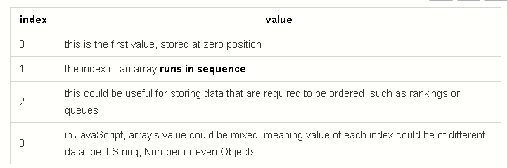
indexvalue0 ... this is the first value, stored at zero position
- The index of an array runs in sequence
2. This could be useful for storing data that are required to be ordered, such as rankings or queues
3. In JavaScript, array's value could be mixed; meaning value of each index could be of different data, be it String, Number or even Objects
view rawarrays.js hosted with ❤ by GitHub
2. Objects
Think of objects as a logical grouping of a bunch of properties.
Properties could be some variable that it's storing or some methods that it's using.
I also visualize an object as a table.
The main difference is that object's "index" need not be numbers and is not necessarily sequenced.

https://gist.github.com/bgoonz/ed42c5c0f3a1a7757b33b437a9ad7129#file-object-js %}
view rawobject.js hosted with ❤ by GitHub
The Hash Table
Definition
A Hash Table (Hash Map) is a data structure used to implement an associative array, a structure that can map keys to values. A Hash Table uses a hash function to compute an index into an array of buckets or slots, from which the desired value can be found. From Wikipedia
Hash Tables are considered the more efficient data structure for lookup and for this reason, they are widely used.
Complexity\
Average\
Access Search Insertion Deletion
- O(1) O(1) O(1)
The code
Note, here I am storing another object for every hash in my Hash Table.
view rawhashtable.js hosted with ❤ by GitHub
The Set
Sets
Sets are pretty much what it sounds like. It's the same intuition as Set in Mathematics. I visualize Sets as Venn Diagrams.

view rawnative-set.js hosted with ❤ by GitHub

Definition
A Set is an abstract data type that can store certain values, without any particular order, and no repeated values. It is a computer implementation of the mathematical concept of a finite Set. From Wikipedia
The Set data structure is usually used to test whether elements belong to set of values. Rather then only containing elements, Sets are more used to perform operations on multiple values at once with methods such as union, intersect, etc...
Complexity\
Average\
Access Search Insertion Deletion
- O(n) O(n) O(n)
The code >
view rawsetADS.js hosted with ❤ by GitHub
The Singly Linked List

Definition
A Singly Linked List is a linear collection of data elements, called nodes pointing to the next node by means of pointer. It is a data structure consisting of a group of nodes which together represent a sequence. Under the simplest form, each node is composed of data and a reference (in other words, a link) to the next node in the sequence.
Linked Lists are among the simplest and most common data structures because it allows for efficient insertion or removal of elements from any position in the sequence.
Complexity\
Average\
Access Search Insertion Deletion\
O(n) O(n) O(1) O(1)
The code
view rawsingly-linked-list.js hosted with ❤ by GitHub
The Doubly Linked List

Definition
A Doubly Linked List is a linked data structure that consists of a set of sequentially linked records called nodes. Each node contains two fields, called links, that are references to the previous and to the next node in the sequence of nodes. From Wikipedia
Having two node links allow traversal in either direction but adding or removing a node in a doubly linked list requires changing more links than the same operations on a Singly Linked List.
Complexity\
Average\
Access Search Insertion Deletion\
O(n) O(n) O(1) O(1)
The code >
view rawdoubly-linked-list.js hosted with ❤ by GitHub
The Stack

Definition
A Stack is an abstract data type that serves as a collection of elements, with two principal operations: push, which adds an element to the collection, and pop, which removes the most recently added element that was not yet removed. The order in which elements come off a Stack gives rise to its alternative name, LIFO (for last in, first out). From Wikipedia
A Stack often has a third method peek which allows to check the last pushed element without popping it.
Complexity\
Average\
Access Search Insertion Deletion\
O(n) O(n) O(1) O(1)
The code >
view rawstack.js hosted with ❤ by GitHub
The Queue

Definition
A Queue is a particular kind of abstract data type or collection in which the entities in the collection are kept in order and the principal operations are the addition of entities to the rear terminal position, known as enqueue, and removal of entities from the front terminal position, known as dequeue. This makes the Queue a First-In-First-Out (FIFO) data structure. In a FIFO data structure, the first element added to the Queue will be the first one to be removed.
As for the Stack data structure, a peek operation is often added to the Queue data structure. It returns the value of the front element without dequeuing it.
Complexity\
Average\
Access Search Insertion Deletion\
O(n) O(n) O(1) O(n)
The code >
view rawqueue.js hosted with ❤ by GitHub
The Tree
Definition
A Tree is a widely used data structure that simulates a hierarchical tree structure, with a root value and subtrees of children with a parent node. A tree data structure can be defined recursively as a collection of nodes (starting at a root node), where each node is a data structure consisting of a value, together with a list of references to nodes (the "children"), with the constraints that no reference is duplicated, and none points to the root node. From Wikipedia
Complexity\
Average\
Access Search Insertion Deletion\
O(n) O(n) O(n) O(n)\
To get a full overview of the time and space complexity of the Tree data structure, have a look to this excellent Big O cheat sheet.

The code >
view rawbst.js hosted with ❤ by GitHub
The Graph
Definition
A Graph data structure consists of a finite (and possibly mutable) set of vertices or nodes or points, together with a set of unordered pairs of these vertices for an undirected Graph or a set of ordered pairs for a directed Graph. These pairs are known as edges, arcs, or lines for an undirected Graph and as arrows, directed edges, directed arcs, or directed lines for a directed Graph. The vertices may be part of the Graph structure, or may be external entities represented by integer indices or references.
- A graph is any collection of nodes and edges.
- Much more relaxed in structure than a tree.
- It doesn't need to have a root node (not every node needs to be accessible from a single node)
- It can have cycles (a group of nodes whose paths begin and end at the same node)
- Cycles are not always "isolated", they can be one part of a larger graph. You can detect them by starting your search on a specific node and finding a path that takes you back to that same node.
- Any number of edges may leave a given node
- A Path is a sequence of nodes on a graph
Cycle Visual
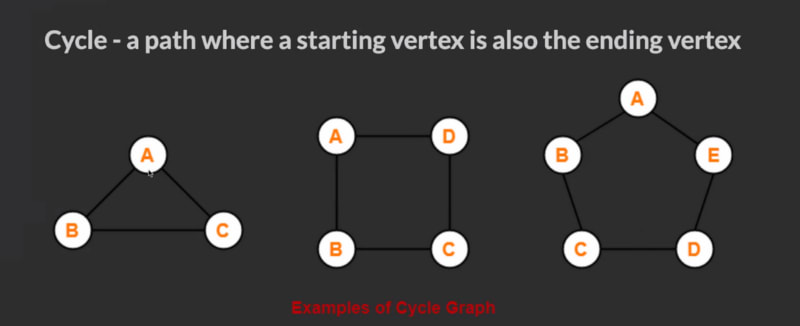
A Graph data structure may also associate to each edge some edge value, such as a symbolic label or a numeric attribute (cost, capacity, length, etc.).
Representation\
There are different ways of representing a graph, each of them with its own advantages and disadvantages. Here are the main 2:
Adjacency list: For every vertex a list of adjacent vertices is stored. This can be viewed as storing the list of edges. This data structure allows the storage of additional data on the vertices and edges.\
Adjacency matrix: Data are stored in a two-dimensional matrix, in which the rows represent source vertices and columns represent destination vertices. The data on the edges and vertices must be stored externally.
Ways to Reference Graph Nodes
Node Class
Uses a class to define the neighbors as properties of each node.
class GraphNode {
  constructor(val) {
    this.val = val;
    this.neighbors = [];
  }
}

let a = new GraphNode("a");
let b = new GraphNode("b");
let c = new GraphNode("c");
let d = new GraphNode("d");
let e = new GraphNode("e");
let f = new GraphNode("f");
a.neighbors = [e, c, b];
c.neighbors = [b, d];
e.neighbors = [a];
f.neighbors = [e];
Adjacency Matrix
The row index will corespond to the source of an edge and the column index will correspond to the edges destination.
- When the edges have a direction,
matrix[i][j]may not be the same asmatrix[j][i] - It is common to say that a node is adjacent to itself so
matrix[x][x]is true for any node - Will be O(n^2) space complexity
let matrix = [

|       | **A**   | **B**  | **C**  | **D**  | **E**  | **F**  |
| ----- | ------- | ------ | ------ | ------ | ------ | ------ |
| **A** | [True,  | True,  | True,  | False, | True,  | False] |
| **B** | [False, | True,  | False, | False, | False, | False] |
| **C** | [False, | True,  | True,  | True,  | False, | False] |
| **D** | [False, | False, | False, | True,  | False, | False] |
| **E** | [True,  | False, | False, | False, | True,  | False] |
| **F** | [False, | False, | False, | False, | True,  | True]  |

];
Adjacency List
Seeks to solve the shortcomings of the matrix implementation. It uses an object where keys represent node labels and values associated with that key are the adjacent node keys held in an array.
let graph = {
  a: ["b", "c", "e"],
  b: [],
  c: ["b", "d"],
  d: [],
  e: ["a"],
  f: ["e"],
};
Code Examples
Basic Graph Class
class Graph {
  constructor() {
    this.adjList = {};
  }

  addVertex(vertex) {
    if (!this.adjList[vertex]) this.adjList[vertex] = [];
  }

  addEdges(srcValue, destValue) {
    this.addVertex(srcValue);
    this.addVertex(destValue);
    this.adjList[srcValue].push(destValue);
    this.adjList[destValue].push(srcValue);
  }

  buildGraph(edges) {
    edges.forEach((ele) => {
      this.addEdges(ele[0], ele[1]);
    });
    return this.adjList;
  }

  breadthFirstTraversal(startingVertex) {
    const queue = [startingVertex];
    const visited = new Set();
    const result = new Array();

    while (queue.length) {
      const value = queue.shift();
      if (visited.has(value)) continue;
      result.push(value);
      visited.add(value);
      queue.push(...this.adjList[value]);
    }
    return result;
  }

  depthFirstTraversalIterative(startingVertex) {
    const stack = [startingVertex];
    const visited = new Set();
    const result = new Array();

    while (stack.length) {
      const value = stack.pop();
      if (visited.has(value)) continue;
      result.push(value);
      visited.add(value);
      stack.push(...this.adjList[value]);
    }
    return result;
  }

  depthFirstTraversalRecursive(
    startingVertex,
    visited = new Set(),
    vertices = []
  ) {
    if (visited.has(startingVertex)) return [];

    vertices.push(startingVertex);
    visited.add(startingVertex);

    this.adjList[startingVertex].forEach((vertex) => {
      this.depthFirstTraversalRecursive(vertex, visited, vertices);
    });
    return [...vertices];
  }
Node Class Examples
class GraphNode {
  constructor(val) {
    this.val = val;
    this.neighbors = [];
  }
}

function breadthFirstSearch(startingNode, targetVal) {
  const queue = [startingNode];
  const visited = new Set();

  while (queue.length) {
    const node = queue.shift();
    if (visited.has(node.val)) continue;
    visited.add(node.val);
    if (node.val === targetVal) return node;
    node.neighbors.forEach((ele) => queue.push(ele));
  }
  return null;
}

function numRegions(graph) {
  let maxLength = 0;
  for (node in graph) {
    if (graph[node].length > maxLength) maxLength = graph[node].length;
  }
  if (maxLength === 0) {
    return (length = Object.keys(graph).length);
  } else {
    return maxLength;
  }
}

function maxValue(node, visited = new Set()) {
  let queue = [node];
  let maxValue = 0;
  while (queue.length) {
    let currentNode = queue.shift();
    if (visited.has(currentNode.val)) continue;
    visited.add(currentNode.val);
    if (currentNode.val > maxValue) maxValue = currentNode.val;
    currentNode.neighbors.forEach((ele) => queue.push(ele));
  }
  return maxValue;
}
Traversal Examples
With Graph Node Class
function depthFirstRecur(node, visited = new Set()) {
  if (visited.has(node.val)) return;

  console.log(node.val);
  visited.add(node.val);

  node.neighbors.forEach((neighbor) => {
    depthFirstRecur(neighbor, visited);
  });
}

function depthFirstIter(node) {
  let visited = new Set();
  let stack = [node];

  while (stack.length) {
    let node = stack.pop();

    if (visited.has(node.val)) continue;

    console.log(node.val);
    visited.add(node.val);

    stack.push(...node.neighbors);
  }
}
With Adjacency List
function depthFirst(graph) {
  let visited = new Set();

  for (let node in graph) {
    _depthFirstRecur(node, graph, visited);
  }
}

function _depthFirstRecur(node, graph, visited) {
  if (visited.has(node)) return;

  console.log(node);
  visited.add(node);

  graph[node].forEach((neighbor) => {
    _depthFirstRecur(neighbor, graph, visited);
  });
}
view rawgraph-representation.md hosted with ❤ by GitHub
Graph
The code
view rawgraph.js hosted with ❤ by GitHub
Memoization & Tabulation (Dynamic Programming)
What is Memoization?
And why this programming paradigm shouldn't make you cringe

 Memoization is a design paradigm used to reduce the overall number of
calculations that can occur in algorithms that use recursive algorithms.
Recall that recursion solves a large problem by dividing it into smaller
sub-problems that are more manageable.
Memoization will store the results of the sub-problems in some other data structure, meaning that you avoid duplicate calculations and only "solve" each subproblem once.
This approach is near synonymous with another computer science term you may have heard before — caching. However, caching as a practice is not achieved exclusively by memoizing. Think of a cache as a little bucket where we will keep important information we don't want to forget in the near future but that isn't vitally important or part of the long-term makeup of our application. It's less important than the things we need to store in memory but more important than a variable we can discard as soon as we use it once.
There are two features that comprise memoization:
- The function is recursive.
- The additional data structure used is typically an object (we refer to this as
the memo).
This is a trade-off between the time it takes to run an algorithm (without
memoization) and the memory used to run the algorithm (with memoization).
Usually, memoization is a good trade-off when dealing with large data or
calculations.
You cannot always apply this technique to recursive problems. The problem must have an "overlapping subproblem structure" for memoization to be effective.
Generally speaking, computer memory is cheap and human time is incalculably valuable so we may opt for this approach even when the largest gains on paper can be made from converting RAM at the expense of execution speed.
Here's an example of a problem that has such a structure:
Using pennies, nickels, dimes, and quarters, how many combinations
of coins are there that total 27 cents?
Along the way to calculating the possible coin combination of 27
cents, you should also calculate the smallest coin combination of 25 cents as well as 21 cents and any smaller total that comprises a fraction of the total combination of 27 (so long as there is a one-cent piece; if there are only nickels and up, the problem deviates from this approach on a technicality but in essence, it is still calculated in the same manner, that is to say as a component of that bigger problem).
Remember, a computer is stupid and must check every possibility exhaustively to ensure that no possible combination is missed (in reality, I may be oversimplifying the truth of the matter but for now, please bear with me).
This is the essence of a redundant subcomponent of the overall problem.
Memoizing factorial
From this plain factorial above, it is clear that every time you call
factorial(6) you should get the same result of 720 each time. The code is
somewhat inefficient because you must go down the full recursive stack for each top-level call to factorial(6).
If we can store the result of factorial(6) the first time you calculate it, then on subsequent calls to factorial(6) you simply fetch the stored result in constant time.
The memo object above will map an argument of factorial to its return
value. That is, the keys will be arguments and their values will be the
corresponding results returned. By using the memo, you are able to avoid
duplicate recursive calls!
By the time your first call to factorial(6)returns, you will not have just the argument 6 stored in the memo. Rather, y*ou will have all arguments 2 to 6 stored in the memo.*
Perhaps you're not convinced because:
- You didn't improve the speed of the algorithm by an order of Big-O (it is
still O(n)). - The code uses some global variable, so it's kind of ugly.
Memoizing the Fibonacci generator
Here's a naive implementation of a function that calculates the Fibonacci
number for a given input.
function fib(n) {
  if (n === 1 || n === 2) return 1;
  return fib(n - 1) + fib(n - 2);
}

fib(6);     // => 8
The time complexity of this function is not super intuitive to describe because
the code branches twice recursively. Fret not! You'll find it useful to
visualize the calls needed to do this with a tree. When reasoning about the time complexity for recursive functions, draw a tree that helps you see the calls. Every node of the tree represents a call of the recursion:
 - *n *, the height of this tree will be
 n. You derive this by following
the path going straight down the left side of the tree.
- each internal node leads to two more nodes. Overall, this means that the tree will have roughly 2n nodes.
- which is the same as saying that the
fibfunction has an exponential time complexity of 2n. - That is very slow!
See for yourself, try running fib(50) - you'll be waiting for quite a lot longer than you've gotten used to waiting for a program to run in the last decade.
The green regions highlighted above are repetitive.
As the n grows bigger, the number of duplicate sub-trees grows exponentially.
Luckily you can fix this using memoization by using a similar object strategy.
You can use some JavaScript default arguments memo={} to clean things up:
You can see the marked nodes (function calls) that access the memo in green.
It's easy to see that this version of the Fibonacci generator will do far fewer
computations as n grows larger! In fact, this memoization has brought the time complexity down to linear O(n) time because the tree only branches on the left side. This is an enormous gain if you recall the complexity of class hierarchy.
The memoization formula
Now that you understand memoization, when should you apply it? Memoization is useful when attacking recursive problems that have many overlapping sub-problems.
You'll find it most useful to draw out the visual tree first. If you notice duplicate sub-trees, time to memoize. Here are the hard and fast
rules you can use to memoize a slow algorithm:
- Write the unoptimized, brute force recursion and make sure it works.
- Add the memo object as an additional argument to the function. The keys will
represent unique arguments to the function, and their values will represent the results for those arguments. - Add a base case condition to the function that returns the stored value if
the function's argument is in the memo. - Before you return the result of the recursive case, store it in the memo as a
value and make the function's argument its key.
Practice:
//! In tabulation we create a table(array) and fill it with elements.
// We will complete the table by filling entries from first to last, or "left to right".
// -->This means that the first entry of the table(first element of the array) will correspond to the smallest subproblem.
// ---->The final entry of the table(last element of the array) will correspond to the largest problem !!(which is also the final answer.)!!
// There are two main features that comprise the Tabulation strategy:
// //1. the function is iterative and not recursive
//// 2. the additional data structure used is typically an array, commonly referred to as the table
// Example:
// Once again, we will use the fibonacci example for demonstration
function tabulatedFib(n) {
  // !create a blank array with n reserved spots
  let table = new Array(n);
  //console.log(table);
  //! initialize the first two values
  table[0] = 0;
  table[1] = 1;
  // complete the table by moving from left to right,

  for (let i = 2; i <= n; i += 1) {
    table[i] = table[i - 1] + table[i - 2];
    //console.log(table);
  }
  ////console.log(table);
  return table[n];
}
//console.log("tabulatedFib(6): ", tabulatedFib(6));
//console.log("tabulatedFib(7): ", tabulatedFib(7));
/*
bryan@LAPTOP-F699FFV1:/mnt/c/Users/15512/Google Drive/a-A-September/weeks/week-7/days/tuesday/Past-Cohort/Useful$ node algos.js
[ <6 empty items> ]
[ 0, 1, 1, <3 empty items> ]
[ 0, 1, 1, 2, <2 empty items> ]
[ 0, 1, 1, 2, 3, <1 empty item> ]
[ 0, 1, 1, 2, 3, 5 ]
[0, 1, 1, 2, 3, 5, 8]
[ 0, 1, 1, 2, 3, 5, 8]
-tabulatedFib(6):  8
[ <7 empty items> ]
[ 0, 1, 1, <4 empty items> ]
[ 0, 1, 1, 2, <3 empty items> ]
[ 0, 1, 1, 2, 3, <2 empty items> ]
[ 0, 1, 1, 2, 3, 5, <1 empty item> ]
[0, 1, 1, 2,3, 5, 8]
[ 0, 1, 1,  2, 3, 5, 8, 13]
[ 0, 1, 1,  2, 3, 5, 8, 13]
-tabulatedFib(7):  13
*/
// console.log(tabulatedFib(7));      // => 13
// When we initialize the table and seed the first two values, it will look like this:
//   i        | 0 | 1 | 2 | 3 | 4 | 5 | 6 | 7 |
// ------------------------------------------
// table[i] | 0 | 1 |   |   |   |   |   |   |
// After the loop finishes, the final table will be:
//   i       | 0 | 1 | 2 | 3 | 4 | 5 | 6 | 7 |
// -----------------------------------------
// table[i]| 0 | 1 | 1 | 2 | 3 | 5 | 8 | 13|

//// Bonus:
//? ------------------HOW DOES THIS WORK--------------------------------
//! MOORE's LAWWWWWWWWWWWWWWWWW!!!!!!!!!!!
//! This is NOT tabulation, but an improvement on the code we just wrote.
//1, 2, 3, 5, (8), 13, 21
//fib(5)=8
//[0,1]

function SpaceSavingFib(n) {
  let mostRecentFibs = [0, 1];
  if (n === 0) return mostRecentFibs[0]; //0
  for (let i = 2; i <= n; i++) {
    // because values are alredy in table
    const [secondLast, last] = mostRecentFibs; //destructure
    mostRecentFibs = [last, secondLast + last]; //? how does this work?
  }
  return mostRecentFibs[1];
}
//console.log("SpaceSavingFib(6): ", SpaceSavingFib(6)); //-SpaceSavingFib(6):  8
//?  ------------------------------------END OF CONFUSION LOL --------------

//// Word break-------------------------------------------------------------
/*
The fill() method changes all elements in an array to a static value, from a start index (default 0) to an end index (default array.length).
It returns the modified array.
Syntax
arr.fill(value[, start[, end]])
Parameters
!value
-Value to fill the array with. (Note all elements in the array will be this exact value.)
?start Optional
-Start index, default 0.
?end Optional
-End index, default arr.length.

!Return value
-The modified array, filled with value.

Description
If start is negative, it is treated as array.length + start.
If end is negative, it is treated as array.length + end.
fill is intentionally generic: it does not require that its this value be an Array object.
fill is a mutator method: it will change the array itself and return it, not a copy of it.
If the first parameter is an object, each slot in the array will reference that object.
*/
function wordBreak(string, dictionary) {
  //! "gooddog", ["good", "dog"]

  ////The fill() method changes all elements in an array to a static value ⬆️, from a start index (default 0) to an end index (default array.length).
  ////It returns the modified array.

  let table = new Array(string.length + 1).fill(false); //-[false, false, false, false, false, false, false, false];
  table[0] = true; //-[true, false, false, false, false, false, false, false];
  for (let i = 0; i < table.length; i++) {
    if (table[i] === false) continue; //-table[0] = true, table[4] = true
    //console.log(table); // [ true,  false, false, false, true,  false, false, true]
    for (let j = i + 1; j < table.length; j++) {
      //*Unique Pairs
      let word = string.slice(i, j); //testing every combination of subsets of the string
      if (dictionary.includes(word)) table[j] = true; //table[4], table[8] = true
      //console.log(table);
    }
  }
  return table[table.length - 1];
}
const dictionary = ["good", "dog"];
const string = "gooddog";
// wordBreak( string, dictionary );
// console.log( wordBreak( string, dictionary ) ); //!true

//------------------------Annagram----------------------------------------------------------------------------------------------------------------------------
/*
!Anagrams
Our goal today is to write a method that determines if two given words are anagrams(the letters in one word can be rearranged to form the other word).
For example:
-->anagram("gizmo", "sally")    # => false
-->anagram("elvis", "lives")    # => true
Assume that there is no whitespace or punctuation in the given strings.
Phase 4;
Write one more method fourth_anagram.This time, use two objects to store the
number of times each letter appears in both words.
Compare the resulting objects.
What is the time complexity ?
    Bonus : Do it with only one object.
Discuss the time complexity of your solutions together, then call over your TA to look at them.
*/
function anagrams(str1, str2) {
  if (str1.length !== str2.length) return false; // if the lengths of the strings differ they cannot possibly be anagrams

  let count = {};

  for (let i = 0; i < str1.length; i++) {
    //---------------------String1-----------------------------------------------------------
    if (count[str1[i]] === undefined) {
      // if the string does not exist in the object
      count[str1[i]] = 0; //initialize the string as a key (and value 0)
    }
    count[str1[i]] += 1; // increase the value for that key by 1
    //--------------------string2------------------------------------------------------------
    if (count[str2[i]] === undefined) {
      // if the second string does not exist in the object
      count[str2[i]] = 0; //initialize the string as a key (and value 0)
    }
    count[str2[i]] -= 1;
    console.log(count);
    //--------------End of Loop--------------------------------------------------------------
  }
  // console.log(count);
  return Object.values(count).every((num) => {
    return num === 0;
  });
}
const str1 = "asdfgh";
const str2 = "hgfdsa";
//console.log(anagrams(str1, str2));
/*
{ a: 1, h: -1 }
{ a: 1, h: -1, s: 1, g: -1 }
{ a: 1, h: -1, s: 1, g: -1, d: 1, f: -1 }
{ a: 1, h: -1, s: 1, g: -1, d: 0, f: 0 }
{ a: 1, h: -1, s: 0, g: 0, d: 0, f: 0 }
{ a: 0, h: 0, s: 0, g: 0, d: 0, f: 0 }
true
*/
const str3 = "asdfghh";
const str4 = "hgfdsaa";
//console.log(anagrams(str3, str4));
/*
{ a: 1, h: -1 }
{ a: 1, h: -1, s: 1, g: -1 }
{ a: 1, h: -1, s: 1, g: -1, d: 1, f: -1 }
{ a: 1, h: -1, s: 1, g: -1, d: 0, f: 0 }
{ a: 1, h: -1, s: 0, g: 0, d: 0, f: 0 }
{ a: 0, h: 0, s: 0, g: 0, d: 0, f: 0 }
{ a: -1, h: 1, s: 0, g: 0, d: 0, f: 0 }
false
*/

// //-----------Anagram Walkthrough----------Uncomment-----------------------------
// function anagrams(str1, str2) {
//   if (str1.length !== str2.length) return false; // if the lengths of the strings differ they cannot possibly be anagrams
//
//   let count = {};
//   /*
// const str1 = "asdfgh";
// const str2 = "hgfdsa";
// */
//   //! when i = 0
//   //*when i = 1
//   //// when i = 2
//   //?when i = 3
//
//   for (let i = 0; i < str1.length; i++) {
//     //---------------------String1-----------------------------------------------------------
//     if (count[str1[i]] === undefined) {
//       //! true
//       //*true
//       ////true
//       //? FALSE
//       // if the string does not exist in the object
//       count[str1[i]] = 0; //! count = {"a":0}
//       //*{ a: 1, h: -1, s: 0,}
//       ////{ a: 1, h: -1, s: 1, g: -1, d: 0}
//       //? DOES NOT HAPPEN
//     }
//     count[str1[i]] += 1; //! count = {"a":1}
//     //*{ a: 1, h: -1, s: 1,}
//     ////{ a: 1, h: -1, s: 1, g: -1, d: 1}
//     //?
//     //--------------------string2------------------------------------------------------------
//     if (count[str2[i]] === undefined) {
//       //! true
//       //*true
//       ////true
//       //? FALSE
//       // if the second string does not exist in the object
//       count[str2[i]] = 0; //! count = {"a":0, "h":0}
//       //*{ a: 1, h: -1, s: 1, g: 0 }
//       ////{ a: 1, h: -1, s: 1, g: -1, d: 1, f: 0 }
//       //? { a: 1, h: -1, s: 1, g: -1, d: 1, f: 0 }  <----- f= 0 ... (!!!the f in each word cancels out!!!)
//     }
//     count[str2[i]] -= 1; //! count = {"a":0, "h":-1}
//     //*{ a: 1, h: -1, s: 1, g: -1 }
//     ////{ a: 1, h: -1, s: 1, g: -1, d: 1, f: -1 }
//     //?
//     console.log(count); //# Same as count object directly above this log statment
//
//     //--------------End of Loop--------------------------------------------------------------
//   }
//   // console.log(count);
//   return Object.values(count).every((num) => {
//     return num === 0;
//   });
// }
// const str1 = "asdfgh";
// const str2 = "hgfdsa";
// console.log(anagrams(str1, str2));//!true
//
// const str3 = "asdfghh";
// const str4 = "hgfdsaa";
// console.log(anagrams(str3, str4));//!false

//****************************END OF ANAGRAM***************************************************** */

//!  ***************************************MEMOIZATION*******************************************/*
/*
Memoization is a design pattern used to reduce the overall number of calculations in algorithms that use recursive strategies.
//Memoization will store the results of the sub-problems in some other data structure.
There are two features that comprise memoization:
-1. the function is recursive
-2. the additional data structure used is typically an object(we refer to this as the memo!) (or cache!)
Example:
Our fibonacci fucntions have two recursive calls.
- time complexity of O(2^n)
*/
function slowFib(n) {
  if (n === 1 || n === 2) return 1;
  return slowFib(n - 1) + slowFib(n - 2);
}
//slowFib(6);
//console.log("slowFib(6): ", slowFib(6)); //- slowFib(6):  8
//---------------------------------------------------------------------------------------------------
//                                         f(6)
//                     f(5)                  |                  f(4)
//           f(4)        |         f(3)      |        f(3)       |     f(2)      |
//    f(3)     |  f(2)   |   f(2)   |  f(1)  |   f(2)  |   f(1)  |
// f(2) | f(1) |
// Many of the recursive function calls are being made multiple times
//---------------------------------------------------------------------------------------------------
//! If we store these results in an object,we can reduce the number of recursive calls the function will make.

function fastFib(n, memo = { 1: 1, 2: 1 }) {
  if (n in memo) return memo[n];
  // if (n === 1 || n === 2) return 1;
  memo[n] = fastFib(n - 1, memo) + fastFib(n - 2, memo);
  return memo[n];
}
console.table([
  { "fastFib(4): ": fastFib(4) },
  { "fastFib(6): ": fastFib(6) },
  { "fastFib(50): ": fastFib(50) },
]);
/*
┌─────────┬──────────────┬──────────────┬───────────────┐
│ (index) │ fastFib(4):  │ fastFib(6):  │ fastFib(50):  │
├─────────┼──────────────┼──────────────┼───────────────┤
│    0    │      3       │              │               │
│    1    │              │      8       │               │
│    2    │              │              │  12586269025  │
└─────────┴──────────────┴──────────────┴───────────────┘
*/

/*
//fastFib(6); // => 8
//fastFib(50); // => 12586269025
Before memoization
                                        f(6)
                    f(5)                  |                  f(4)
          f(4)        |         f(3)      |        f(3)       |     f(2)      |
   f(3)     |  f(2)   |   f(2)   |  f(1)  |   f(2)  |   f(1)  |
f(2) | f(1) |
--------------------------------------------------------------------------------------
Now, our function calls will look like this:
                                        f(6)
                    f(5)                  |           f(4) <= retrieve stored answer
          f(4)        |         f(3)   <= retrieve stored answer
   f(3)     |  f(2)   |
f(2) | f(1) |
-In slowFib, the number of procedures is about 2^n, giving a time complexity of O(2^n)
-In fastFib, the number of procedures is 1+2(n-2) = 2n-3, giving a time complexity of O(n)
*/

Top comments (0)