
This blog is Part One of a multi-part series that highlights the Excel 2019 functions and shows how to create an Air Quality Index report (AQI) using GcExcel API.
With the abundance of data available to businesses today, it becomes even more important to find efficient ways to analyze and process this data in meaningful ways. Spreadsheets are a powerful way to manage this. Specifically, by using functions, complex calculations can be created to save time, money and ultimately provide a robust analysis of large data sets.
With the Microsoft Excel 2019 release, six new functions are introduced, simplifying some common calculations:
- The CONCAT function can be used to combine multiple string values, including values in cell ranges.
- The TEXTJOIN function can also be used to combine multiple string values, including values in cell ranges. Additionally, it lets you specify a delimiter and choose whether to ignore empty cells.
- The IFS function can evaluate multiple conditions to return a value that corresponds to the first TRUE condition.
- The SWITCH function can be used to evaluate one value (known as an expression) against a list of value-result pairs, to return the result corresponding to the first matching value.
- The MAXIFS function can be used to return the maximum value among cells specified by a given set of conditions or criteria.
- The MINIFS function can be used to return the minimum value among cells specified by a given set of conditions or criteria.
All these above functions are supported by GrapeCity Documents for Excel library, referred to as GcExcel.
GcExcel is a high-performance spreadsheet solution that provides a comprehensive API to quickly create, manipulate, convert, and share Microsoft Excel-compatible spreadsheets. Refer to this quick tutorial on how to get started with GcExcel.
Let’s take a look at how to implement these functions in GcExcel to achieve a real-world scenario.
Use Case: Air Quality Index Report
An Air Quality Index (AQI) is an indicator to measure air quality in a particular area or region. In this blog, we will create an AQI Report using the newly introduced functions in GcExcel, to display the Air Quality Index of 10 capital cities across different countries and 4 major cities of the US.
Data Source
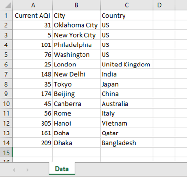
The below data is added to the “Data” worksheet in a workbook saved as an Excel file using GcExcel.
Here is a sample code snippet for adding the above data in GcExcel:
//Define source data
object[,] sourceData = new object[,] {
{ "Current AQI", "City", "Country"},
{ 31, "Oklahoma City","US"},
{ 5, "New York City","US"},
{ 101, "Philadelphia","US"},
{ 76, "Washington",  "US"},
{ 25, "London",  "United Kingdom"},
{ 148, "New Delhi",  "India"},
{ 35, "Tokyo",  "Japan"},
{ 174, "Beijing",  "China"},
{ 45, "Canberra",  "Australia"},
{ 56, "Rome", "Italy"},
{ 305, "Hanoi", "Vietnam"},
{ 161, "Doha", "Qatar"},
{ 209, "Dhaka","Bangladesh"}
};

//Add new worksheet and name it as 'Data'
var workbook = new GrapeCity.Documents.Excel.Workbook();
IWorksheet worksheet = workbook.Worksheets[0];
worksheet.Name = "Data";

//Add source data
worksheet.Range["A1:C14"].Value = sourceData;
It will be used as the data source to create the AQI Report, as explained in the below section.
AQI Report
The AQI report uses the above-mentioned data and implements functions over it to display the following:
- The Location column displays the combination of “City” and “Country” columns using TEXTJOIN/CONCAT functions.
- The Current AQI column, which displays the AQI values straight from the ‘Current AQI’ column.
- The Level of Health Concern column displays the severity of health concerns using IFS/SWITCH functions.
Apart from the above, the AQI report also displays the US cities with the worst and best AQI by using the MAXIFS and MINIFS functions, respectively. Here is a quick look at how the final AQI Report will look:

The color scheme applied to the AQI report in the above image is done with the help of another useful feature of GcExcel, known as conditional formatting. Please refer to Conditional Formatting in GcExcel documentation for more details.
Note: The same AQI report is created in two separate worksheets, namely, “TEXTJOIN&IFS” and “CONCAT&SWITCH”, to showcase the usage of similar functions achieving the same output.
Now that we have seen the final product, let's dive into the details of implementing these functions.
Generating Location List
The "Location" column values in the AQI report are generated by using either TEXTJOIN or CONCAT functions.
TEXTJOIN Function
The TEXTJOIN function helps combine text from multiple ranges and/or strings. It also provides the ‘delimiter’ and ‘ignoreempty’ arguments:
Syntax: TEXTJOIN(delimiter, ignoreempty, text1, [text2], ...)
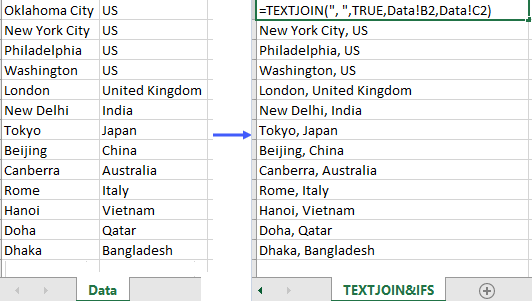
We have applied the TEXTJOIN function in the “TEXTJOIN&IFS” worksheet to combine the “City” and “Country” columns of the “Data” sheet. Here, a comma is used as a delimiter, and ignore empty cells is set to true.
Here is a sample code snippet for using the TEXTJOIN function in GcExcel:
//Apply TEXTJOIN function
worksheet1.Range["A4"].Formula = "=TEXTJOIN(\", \", true, Data!B2, Data!C2)";
worksheet1.Range["A5"].Formula = "=TEXTJOIN(\", \", true, Data!B3, Data!C3 )";
worksheet1.Range["A6"].Formula = "=TEXTJOIN(\", \", true, Data!B4, Data!C4 )";
worksheet1.Range["A7"].Formula = "=TEXTJOIN(\", \", true, Data!B5, Data!C5 )";
worksheet1.Range["A8"].Formula = "=TEXTJOIN(\", \", true, Data!B6, Data!C6 )";
worksheet1.Range["A9"].Formula = "=TEXTJOIN(\", \", true, Data!B7, Data!C7 )";
worksheet1.Range["A10"].Formula = "=TEXTJOIN(\", \", true, Data!B8, Data!C8 )";
worksheet1.Range["A11"].Formula = "=TEXTJOIN(\", \", true, Data!B9, Data!C9 )";
worksheet1.Range["A12"].Formula = "=TEXTJOIN(\", \", true, Data!B10, Data!C10 )";
worksheet1.Range["A13"].Formula = "=TEXTJOIN(\", \", true, Data!B11, Data!C11 )";
worksheet1.Range["A14"].Formula = "=TEXTJOIN(\", \", true, Data!B12, Data!C12 )";
worksheet1.Range["A15"].Formula = "=TEXTJOIN(\", \", true, Data!B13, Data!C13 )";
worksheet1.Range["A16"].Formula = "=TEXTJOIN(\", \", true, Data!B14, Data!C14 )";
The output looks like this after applying the TEXTJOIN function:
CONCAT Function
The CONCAT function helps to combine text from multiple ranges and/or strings:
Syntax: CONCAT(text1, [text2], ...)
We have applied the CONCAT function in the “CONCAT&SWITCH” worksheet to achieve the same output as the TEXTJOIN function. As already mentioned, the CONCAT function does not provide an option to specify a delimiter. Hence, the delimiter is also provided as a text argument which will be concatenated like other text values.
Here is a sample code snippet for using the CONCAT function in GcExcel:
//Apply CONCAT function
worksheet2.Range["A4"].Formula = "=CONCAT(Data!B2, \", \", Data!C2)";
worksheet2.Range["A5"].Formula = "=CONCAT(Data!B3,  \", \", Data!C3 )";
worksheet2.Range["A6"].Formula = "=CONCAT(Data!B4, \", \", Data!C4 )";
worksheet2.Range["A7"].Formula = "=CONCAT(Data!B5, \", \", Data!C5 )";
worksheet2.Range["A8"].Formula = "=CONCAT(Data!B6,  \", \",Data!C6 )";
worksheet2.Range["A9"].Formula = "=CONCAT(Data!B7, \", \", Data!C7 )";
worksheet2.Range["A10"].Formula = "=CONCAT(Data!B8, \", \", Data!C8 )";
worksheet2.Range["A11"].Formula = "=CONCAT(Data!B9,  \", \",Data!C9 )";
worksheet2.Range["A12"].Formula = "=CONCAT(Data!B10, \", \", Data!C10 )";
worksheet2.Range["A13"].Formula = "=CONCAT(Data!B11, \", \", Data!C11 )";
worksheet2.Range["A14"].Formula = "=CONCAT(Data!B12, \", \", Data!C12 )";
worksheet2.Range["A15"].Formula = "=CONCAT(Data!B13, \", \", Data!C13 )";
worksheet2.Range["A16"].Formula = "=CONCAT(Data!B14, \", \", Data!C14 )";
Which one to choose?
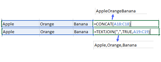
TEXTJOIN is the better candidate as it provides more flexibility and functionality than the CONCAT function. TEXTJOIN provides the delimiter and ignoreempty arguments as additional options. Here is an example to understand this better:
Evaluating Health Concern Levels
The values for the "Level of Health Concern" column in the AQI report can be evaluated by using either IFS or SWITCH functions.
The table below shows how the “Level of Health Concern” is evaluated based on where the value of the current AQI falls within specific ranges. These range values act as criteria for the conditions or expressions passed to IFS and SWITCH functions.

IFS Function
The IFS function helps to check whether one or more conditions are met and returns a value that corresponds to the first TRUE condition:
Syntax: IFS(condition1, truevalue1, [condition2, truevalue2], ...)
We have applied the IFS function in the “TEXTJOIN&IFS” worksheet to evaluate multiple conditions that identify the range in which the Current AQI value falls and returns the corresponding result.
Here is a sample code snippet for using the IFS function in GcExcel:
//Apply IFS function
worksheet1.Range["C4"].Formula = "=IFS(B4>300, \"Hazardous\", B4>200, \"Very Unhealthy\", B4>150, \"Unhealthy\", B4>100, \"Moderate\", B4>50, \"Satisfactory\", B4<=50, \"Good\")";
worksheet1.Range["C5"].Formula = "=IFS(B5>300, \"Hazardous\", B5>200, \"Very Unhealthy\", B5>150, \"Unhealthy\", B5>100, \"Moderate\", B5>50, \"Satisfactory\", B5<=50, \"Good\")";
worksheet1.Range["C6"].Formula = "=IFS(B6>300, \"Hazardous\", B6>200, \"Very Unhealthy\", B6>150, \"Unhealthy\", B6>100, \"Moderate\", B6>50, \"Satisfactory\", B6<=50, \"Good\")";
worksheet1.Range["C7"].Formula = "=IFS(B7>300, \"Hazardous\", B7>200, \"Very Unhealthy\", B7>150, \"Unhealthy\", B7>100, \"Moderate\", B7>50, \"Satisfactory\", B7<=50, \"Good\")";
worksheet1.Range["C8"].Formula = "=IFS(B8>300, \"Hazardous\", B8>200, \"Very Unhealthy\", B8>150, \"Unhealthy\", B8>100, \"Moderate\", B8>50, \"Satisfactory\", B8<=50, \"Good\")";
worksheet1.Range["C9"].Formula = "=IFS(B9>300, \"Hazardous\", B9>200, \"Very Unhealthy\", B9>150, \"Unhealthy\", B9>100, \"Moderate\", B9>50, \"Satisfactory\", B9<=50, \"Good\")";
worksheet1.Range["C10"].Formula = "=IFS(B10>300, \"Hazardous\", B10>200, \"Very Unhealthy\", B10>150, \"Unhealthy\", B10>100, \"Moderate\", B10>50, \"Satisfactory\", B10<=50, \"Good\")";
worksheet1.Range["C11"].Formula = "=IFS(B11>300, \"Hazardous\", B11>200, \"Very Unhealthy\", B11>150, \"Unhealthy\", B11>100, \"Moderate\", B11>50, \"Satisfactory\", B11<=50, \"Good\")";
worksheet1.Range["C12"].Formula = "=IFS(B12>300, \"Hazardous\", B12>200, \"Very Unhealthy\", B12>150, \"Unhealthy\", B12>100, \"Moderate\", B12>50, \"Satisfactory\", B12<=50, \"Good\")";
worksheet1.Range["C13"].Formula = "=IFS(B13>300, \"Hazardous\", B13>200, \"Very Unhealthy\", B13>150, \"Unhealthy\", B13>100, \"Moderate\", B13>50, \"Satisfactory\", B13<=50, \"Good\")";
worksheet1.Range["C14"].Formula = "=IFS(B14>300, \"Hazardous\", B14>200, \"Very Unhealthy\", B14>150, \"Unhealthy\", B14>100, \"Moderate\", B14>50, \"Satisfactory\", B14<=50, \"Good\")";
worksheet1.Range["C15"].Formula = "=IFS(B15>300, \"Hazardous\", B15>200, \"Very Unhealthy\", B15>150, \"Unhealthy\", B15>100, \"Moderate\", B15>50, \"Satisfactory\", B15<=50, \"Good\")";
worksheet1.Range["C16"].Formula = "=IFS(B16>300, \"Hazardous\", B16>200, \"Very Unhealthy\", B16>150, \"Unhealthy\", B16>100, \"Moderate\", B16>50, \"Satisfactory\", B16<=50, \"Good\")";
Here is the data after applying the IFS function:

SWITCH Function
The SWITCH function helps to evaluate one value (called the expression) against a list of values and returns the result corresponding to the first matching value:
Syntax: SWITCH(expression, value1, result1, [default or value2, result2] ...)
We have applied the SWITCH function in the “CONCAT&SWITCH” worksheet to achieve the same output as the IFS function. As can be observed through the code snippet given below, the SWITCH function specifies the value of expression as “True”.
Further, it evaluates multiple conditions to identify the range in which the Current AQI value falls and returns the result corresponding to the first condition that holds True (as the expression suggests).
Here is a sample code snippet for using the SWITCH function in GcExcel:
//Apply SWITCH function
worksheet2.Range["C4"].Formula = "=SWITCH(true, B4>300, \"Hazardous\", B4>200, \"Very Unhealthy\", B4>150, \"Unhealthy\", B4>100, \"Moderate\", B4>50, \"Satisfactory\", B4<=50, \"Good\")";
worksheet2.Range["C5"].Formula = "=SWITCH(true, B5>300, \"Hazardous\", B5>200, \"Very Unhealthy\", B5>150, \"Unhealthy\", B5>100, \"Moderate\", B5>50, \"Satisfactory\", B5<=50, \"Good\")";
worksheet2.Range["C6"].Formula = "=SWITCH(true, B6>300, \"Hazardous\", B6>200, \"Very Unhealthy\", B6>150, \"Unhealthy\", B6>100, \"Moderate\", B6>50, \"Satisfactory\", B6<=50, \"Good\")";
worksheet2.Range["C7"].Formula = "=SWITCH(true, B7>300, \"Hazardous\", B7>200, \"Very Unhealthy\", B7>150, \"Unhealthy\", B7>100, \"Moderate\", B7>50, \"Satisfactory\", B7<=50, \"Good\")";
worksheet2.Range["C8"].Formula = "=SWITCH(true, B8>300, \"Hazardous\", B8>200, \"Very Unhealthy\", B8>150, \"Unhealthy\", B8>100, \"Moderate\", B8>50, \"Satisfactory\", B8<=50, \"Good\")";
worksheet2.Range["C9"].Formula = "=SWITCH(true, B9>300, \"Hazardous\", B9>200, \"Very Unhealthy\", B9>150, \"Unhealthy\", B9>100, \"Moderate\", B9>50, \"Satisfactory\", B9<=50, \"Good\")";
worksheet2.Range["C10"].Formula = "=SWITCH(true, B10>300, \"Hazardous\", B10>200, \"Very Unhealthy\", B10>150, \"Unhealthy\", B10>100, \"Moderate\", B10>50, \"Satisfactory\", B10<=50, \"Good\")";
worksheet2.Range["C11"].Formula = "=SWITCH(true, B11>300, \"Hazardous\", B11>200, \"Very Unhealthy\", B11>150, \"Unhealthy\", B11>100, \"Moderate\", B11>50, \"Satisfactory\", B11<=50, \"Good\")";
worksheet2.Range["C12"].Formula = "=SWITCH(true, B12>300, \"Hazardous\", B12>200, \"Very Unhealthy\", B12>150, \"Unhealthy\", B12>100, \"Moderate\", B12>50, \"Satisfactory\", B12<=50, \"Good\")";
worksheet2.Range["C13"].Formula = "=SWITCH(true, B13>300, \"Hazardous\", B13>200, \"Very Unhealthy\", B13>150, \"Unhealthy\", B13>100, \"Moderate\", B13>50, \"Satisfactory\", B13<=50, \"Good\")";
worksheet2.Range["C14"].Formula = "=SWITCH(true,B14>300, \"Hazardous\", B14>200, \"Very Unhealthy\", B14>150, \"Unhealthy\", B14>100, \"Moderate\", B14>50, \"Satisfactory\", B14<=50, \"Good\")";
worksheet2.Range["C15"].Formula = "=SWITCH(true,B15>300, \"Hazardous\", B15>200, \"Very Unhealthy\", B15>150, \"Unhealthy\", B15>100, \"Moderate\", B15>50, \"Satisfactory\", B15<=50, \"Good\")";
worksheet2.Range["C16"].Formula = "=SWITCH(true,B16>300, \"Hazardous\", B16>200, \"Very Unhealthy\", B16>150, \"Unhealthy\", B16>100, \"Moderate\", B16>50, \"Satisfactory\", B16<=50, \"Good\")";
Which one to choose?
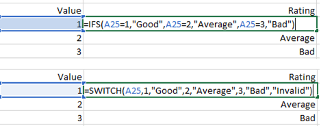
The usage of IFS and SWITCH function generally depends on the usage scenario as explained and shown below:
- The IFS function should be used if the condition-value pairs contain different expressions and operators for each condition
- The SWITCH function should be used if the expression and operator are the same across all conditions to be evaluated. You can also specify a default value in the SWITCH function (‘Invalid’ in the case of the below example) which is returned if there is no match found from the specified conditions.
Displaying Cities with Best and Worst AQI
This section helps in understanding how to evaluate the cities with the worst and best AQI by using MAXIFS and MINIFS functions in “TEXTJOIN&IFS” and “CONCAT&SWITCH” worksheets. These functions are nested with MATCH and INDEX functions to display the desired results.
MAXIFS and MINIFS Functions
The MAXIFS and MINIFS functions help to retrieve the maximum and minimum values among cells specified by a given set of conditions or criteria:
Syntax: MAXIFS(max_range, criteria_range1, criteria1, [criteria_range2, criteria2], ...)
Syntax: MINIFS(min_range, criteria_range1, criteria1, [criteria_range2, criteria2], ...)
We have applied the MAXIFS and MINIFS functions to find the maximum and minimum AQI values from the “Data” sheet where the “Country” value is “US”.
Here is a sample code snippet for using the MAXIFS and MINIFS function in GcExcel. As you can observe, we have also used MATCH and INDEX functions to find out the value of cities with the worst and best AQI:
//Apply MAXIFS and MINIFS functions
worksheet1.Range["B20"].Formula = "=INDEX(Data!B2:B14, MATCH(MAXIFS(Data!A2:A14,Data!C2:C14,\"US\"),Data!A2:A14,0))";
worksheet1.Range["B21"].Formula = "=INDEX(Data!B2:B14, MATCH(MINIFS(Data!A2:A14,Data!C2:C14,\"US\"),Data!A2:A14,0))";
The output looks like this after applying the MAXIFS and MINIFS functions along with other nested functions:

Final AQI Report
//Save workbook
workbook.Save("AQI_Report.xlsx");
This is how the final AQI report looks , in both the worksheets:
- “TEXTJOIN&IFS” Worksheet: Where TEXTJOIN, IFS, and nested MAXIFS and MINIFS functions are used
- “CONCAT&SWITCH” Worksheet: Where CONCAT, SWITCH, and nested MAXIFS and MINIFS functions are used
Try this use case by downloading the sample, which includes all the code snippets described above.
In the Part Two of this blog, we will be covering the charts introduced in Excel 2019 and how to use them in GcExcel.

Top comments (0)