Download the sample MRI dataset from my github . The input images files are in .jpg format and groundtruth is in .xml format. There are missing files to form a complete dataset for segmentation process.
Dataset:
The purpose of the dataset is to provide the research community with a resource to advance the state-of-the-art in image detection, segmentation, and classification as well as help evaluating shortcomings of existing methods. For a labeled region, we provide the location in terms of bounding boxes, classifications. We also provide a detailed description of our annotation pipeline. The results show that some methods achieve excellent detection precision and good transcription accuracy
.Image Processing
Image processing is any form of signal processing for which the input is an image, such as a photograph or video frame, and the output of image processing may be either an image or a set of characteristics or parameters related to the image. Most image processing techniques involve treating the image as a two-dimensional signal and applying standard signal-processing techniques to it.
Image Segmentation
Image segmentation is the process of partitioning an image into multiple segments. Image segmentation is typically used to locate objects and boundaries in images. presents the segmenting result of a femur image. It shows the outer surface (red), the surface between compact bone and spongy bone (green) and the surface of the bone marrow (blue). The testing applied an example of image segmentation to demonstrate the PSO method to find the best clusters of image segmentation. The results showed that PSO runs 170% faster when it used GPU in a parallel mode other than that used CPU alone, for the number of particles 100. This speedup is growing as the number of particles gets higher.
Getting Started:
Importing Packages that we need to execute
import numpy as np
import pandas as pd
from matplotlib import pyplot as plt
import tensorflow as tf
import re
import glob
import matplotlib.pyplot as plt
from matplotlib.patches import Rectangle
import ast
from PIL import Image, ImageDraw
Plotting Function:
the image is defined and arranged in rows and coloumns
plt.subplots()
def image_show(image, nrows=1, ncols=1, cmap='gray'):
    fig, ax = plt.subplots(nrows=nrows, ncols=ncols, figsize=(14, 14))
    ax.imshow(image, cmap='gray')
    ax.axis('off')
    return fig, ax
Function to read in Marks
def read_xml(filename):
    with open(filename, 'r') as f:
        lines = f.readlines()
    return lines
Get a list of files in Thyroid with Segmentatin Coordinates and create list of Image files, segments and Marks
filenames = glob.glob("thyroid/*")
images = [x for x in filenames if x.endswith(".jpg")]
segments = [x for x in filenames if x.endswith(".xml")]
Remove images in which the data does not make sense
pattern = r'"points"(.*?)"annotation"'
segments = segments[segments["mark"].apply(lambda x: len(re.findall(pattern, x))<=2)]
Prepare data for test plot
from ast import literal_eval

# test = segments.loc[segments['img_id']=="thyroid/88_1.jpg"]
test = segments.iloc[0,:]
l = test['mark']#.get_values()[0]
# l = literal_eval(test['mark'])[0]

i = 0
t = 0

test_1 = re.findall(r'\d+', l)

dims = len(test_1)//2

temp = np.empty([dims, 2])
temp

while i < dims:
    temp[i] = (test_1[t], test_1[t+1])
    i = i+1
    t = t+2
Create Plot
fig, ax = image_show(Image.open('thyroid/197_1.jpg'), cmap='gray')
ax.plot(temp[:, 0], temp[:, 1], '.r',lw=3)

Break up Marks for the segmented images
pattern = r'"points"(.*?)"annotation"'
segments["mark_1"] = segments["mark"].apply(lambda x: re.findall(pattern, x)[0])
segments["mark_2"] = segments["mark"].apply(lambda x: re.findall(pattern, x)[1] if len(re.findall(pattern, x)) > 1 else "")
Create temp dataframes and concat
temp_1 = segments[["img_id","mark_1"]].copy()
temp_2 = segments[["img_id","mark_2"]].copy()

temp_1=temp_1.rename(columns = {'mark_1':'mark'})
temp_2=temp_2.rename(columns = {'mark_2':'mark'})

frames = [temp_1, temp_2]

df_new = pd.concat(frames,ignore_index = True)
df_new.head()
Function to parse marks
def parse_mark(mark):
    i = 0
    t = 0
    test_1 = re.findall(r'\d+', mark)
    dims = len(test_1)//2
    temp = np.empty([dims, 2])

    while i < dims:
        temp[i] = (test_1[t], test_1[t+1])
        i = i+1
        t = t+2

    return temp
The final dataset is ready to contain images, masks images, masks inverted images, multi-segmented masks images, outlines images, overlay images, and single_segmented_masks images and it is composed of total 1965.
Unet Model
UNet was first designed especially for medical image segmentation. It showed such good results that it used in many other fields after. In this article, we'll talk about why and how UNet works.

The architecture looks like a ‘U’ which justifies its name. This architecture consists of three sections: The contraction, The bottleneck, and the expansion section. The contraction section is made of many contraction blocks. Each block takes an input that applies two 3X3 convolution layers followed by a 2X2 max pooling. The number of kernels or feature maps after each block doubles so that architecture can learn the complex structures effectively. The bottommost layer mediates between the contraction layer and the expansion layer. It uses two 3X3 CNN layers followed by a 2X2 up convolution layer. Similar to the contraction layer, it also consists of several expansion blocks. Each block passes the input to two 3X3 CNN layers followed by a 2X2 upsampling layer.
Unet Implementation
I implemented the UNet model using the Pytorch framework. You can check out the UNet module for my customized dataset.
Unet_Model
import os
import numpy as np

from skimage.io import imread, imshow, concatenate_images
from skimage.transform import resize
from skimage.morphology import label

import tensorflow as tf

from keras.models import Model, load_model
from keras.layers import Input, BatchNormalization, Activation, Dense, Dropout
from keras.layers.core import Lambda, RepeatVector, Reshape
from keras.layers.convolutional import Conv2D, Conv2DTranspose
from keras.layers.pooling import MaxPooling2D, GlobalMaxPool2D
from keras.layers.merge import concatenate, add
from keras.callbacks import EarlyStopping, ModelCheckpoint, ReduceLROnPlateau
from keras.optimizers import Adam
from keras.preprocessing.image import ImageDataGenerator, array_to_img, img_to_array, load_img
import os
import random
import pandas as pd
import numpy as np
import matplotlib.pyplot as plt
plt.style.use("ggplot")
%matplotlib inline

from tqdm import tqdm_notebook, tnrange
from itertools import chain
from sklearn.model_selection import train_test_split


def conv2d_block(input_tensor, n_filters, kernel_size = 3, batchnorm = True):
    """Function to add 2 convolutional layers with the parameters passed to it"""
    # first layer
    x = Conv2D(filters = n_filters, kernel_size = (kernel_size, kernel_size),\
              kernel_initializer = 'he_normal', padding = 'same')(input_tensor)
    if batchnorm:
        x = BatchNormalization()(x)
    x = Activation('relu')(x)

    # second layer
    x = Conv2D(filters = n_filters, kernel_size = (kernel_size, kernel_size),\
              kernel_initializer = 'he_normal', padding = 'same')(input_tensor)
    if batchnorm:
        x = BatchNormalization()(x)
    x = Activation('relu')(x)

    return x

def get_unet(input_img, n_filters = 8, dropout = 0.2, batchnorm = True):
    """Function to define the UNET Model"""
    # Contracting Path
    c1 = conv2d_block(input_img, n_filters * 1, kernel_size = 3, batchnorm = batchnorm)
    p1 = MaxPooling2D((2, 2))(c1)
    p1 = Dropout(dropout)(p1)

    c2 = conv2d_block(p1, n_filters * 2, kernel_size = 3, batchnorm = batchnorm)
    p2 = MaxPooling2D((2, 2))(c2)
    p2 = Dropout(dropout)(p2)

    c3 = conv2d_block(p2, n_filters * 4, kernel_size = 3, batchnorm = batchnorm)
    p3 = MaxPooling2D((2, 2))(c3)
    p3 = Dropout(dropout)(p3)

    c4 = conv2d_block(p3, n_filters * 8, kernel_size = 3, batchnorm = batchnorm)
    p4 = MaxPooling2D((2, 2))(c4)
    p4 = Dropout(dropout)(p4)

    c5 = conv2d_block(p4, n_filters = n_filters * 16, kernel_size = 3, batchnorm = batchnorm)

    # Expansive Path
    u6 = Conv2DTranspose(n_filters * 8, (3, 3), strides = (2, 2), padding = 'same')(c5)
    u6 = concatenate([u6, c4])
    u6 = Dropout(dropout)(u6)
    c6 = conv2d_block(u6, n_filters * 8, kernel_size = 3, batchnorm = batchnorm)

    u7 = Conv2DTranspose(n_filters * 4, (3, 3), strides = (2, 2), padding = 'same')(c6)
    u7 = concatenate([u7, c3])
    u7 = Dropout(dropout)(u7)
    c7 = conv2d_block(u7, n_filters * 4, kernel_size = 3, batchnorm = batchnorm)

    u8 = Conv2DTranspose(n_filters * 2, (3, 3), strides = (2, 2), padding = 'same')(c7)
    u8 = concatenate([u8, c2])
    u8 = Dropout(dropout)(u8)
    c8 = conv2d_block(u8, n_filters * 2, kernel_size = 3, batchnorm = batchnorm)

    u9 = Conv2DTranspose(n_filters * 1, (3, 3), strides = (2, 2), padding = 'same')(c8)
    u9 = concatenate([u9, c1])
    u9 = Dropout(dropout)(u9)
    c9 = conv2d_block(u9, n_filters * 1, kernel_size = 3, batchnorm = batchnorm)

    outputs = Conv2D(1, (1, 1), activation='sigmoid')(c9)
    model = Model(inputs=[input_img], outputs=[outputs])
    return model
Set Parameters(resize all images in height and width)
im_width = 128
im_height = 128
border = 5
Convert images & masks into arrays
for n, id_ in tqdm_notebook(enumerate(ids), total=len(ids)):
    # Load images
    img = load_img("./data/images/"+id_, grayscale=True)
    x_img = img_to_array(img)
    x_img = resize(x_img, (128, 128, 1), mode = 'constant', preserve_range = True)
    # Load masks
    mask_orig = img_to_array(load_img("./data/masks_inverted/"+id_, grayscale=True))
    mask = resize(mask_orig, (128, 128, 1), mode = 'constant', preserve_range = True)
    # Save images
    X[n] = x_img/255.0
    y[n] = mask/255.0
Split train and valid the dataset
X_train, X_valid, y_train, y_valid = train_test_split(X, y, test_size=0.1, random_state=42)
#Calculate test size ratio
test_size = (X_valid.shape[0]/X_train.shape[0])
# Split train and test
X_train, X_test, y_train, y_test = train_test_split(X_train, y_train, test_size=test_size, random_state=42)
y_train.shape
y_train_plt = y_train.reshape(1571, 128, 128)
import matplotlib.pyplot as plt
plt.imshow(y_train_plt[179, :,:], cmap='gray')
The output has shown below

Plot Loss vs Epoch
plt.figure(figsize=(8, 8))
plt.title("Learning curve")
plt.plot(results.history["loss"], label="loss")
plt.plot(results.history["val_loss"], label="val_loss")
plt.plot( np.argmin(results.history["val_loss"]), np.min(results.history["val_loss"]), marker="x", color="r", label="best model")
plt.xlabel("Epochs")
plt.ylabel("log_loss")
plt.legend();
The output of learning curve is plotted loss vs epoch as shown below

Predictions on test dataset
ix = random.randint(0, len(preds_val))
print(ix)
plot_sample(X_test, y_test, preds_test, preds_test_t,ix=ix)
threshold =.4082
binarize = .1
intersection = np.logical_and(y_test[ix].squeeze() > binarize, preds_test[ix].squeeze() > threshold)
union = np.logical_or(y_test[ix].squeeze() > binarize, preds_test[ix].squeeze() > threshold)
iou=np.sum(intersection) / np.sum(union)
print('IOU:',iou)

Results:
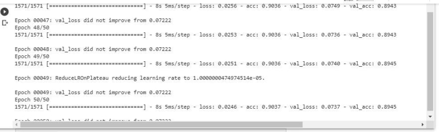
The accuracy of the result is 89.4% from the test dataset.
results = model.fit(X_train, y_train, batch_size=32, epochs=50, callbacks=callbacks,\validation_data=(X_valid, y_valid))

Oldest comments (0)