Mapping Fires using Google Earth Engine and Python

As of recent, several wildfires have ravaged multiple countries for prolonged periods of time, destroying wildlife, imposing collateral damage and overall disrupting multiple natural and anthropogenic processes on an unimaginable scale.

Multiple space agencies across the globe including the ESA (Europe), NASA (United States), CNSA (China), JAXA (Japan) and Roscosmos (Russia) have begun to launch multiple earth-observation satellites from as early as 1957. Recently, the ESA has launched several Earth-Observation satellites as part of their Copernicus programme.

Of particular interest is a pair of sun-synchronous satellites, known collectively as Sentinel-2. Sentinel 2 was launched with the aim to monitor variability in land surface conditions with a relatively short revisit period. Sentinel-2 carries a multi-spectral imaging instrument (or MSI), which is able to passively record 13 spectral bands at 4096 brightness levels.

In other terms, Sentinel-2 can see things our human eyes cannot, by using out-of-visible imaging spectra such as Infrared, Short-Wave Infrared, Red-Edge, etc. The ESA has made much of the data recorded by Sentinel-2 (as well as the entire active and planned Copernicus fleet) freely accessible to the public.

If you are interested in accessing this data directly from the ESA, see this link

Multi-Spectral Imagery and Red-Edge

Sentinel-2 can 'see' multiple frequencies of radiation, including the visible Red, Green and Blue frequencies. This enables Sentinel-2 (and other MSI orbiting platforms) to observe earth-based phenomena at a potentially more discerning level than typical RGB measurements. Moreover, combinations of these bands have been used to extract and classify land-cover using the unique reflectance characteristics of water, types of earth, concrete, etc.

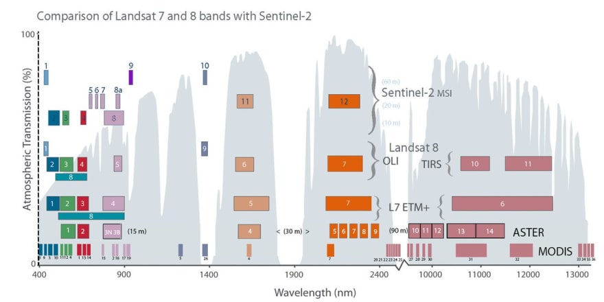
Red-edge is the common name for the sharp change in leaf reflectance between 680nm and 750nm. It is a key length range in remote sensing, that is sensitive to vegetation conditions and can be used to support difference vegetation parameter retrieval products.

In the image below, the red edge is highlighted, and the sharp gradient in this region of the spectrum of imaging bands is clearly apparent. This sharp increase in reflectance at these frequencies by plants (specifically chlorophyll-rich varieties) can be exploited to map potential changes in vegetation.

Burn Severity

Burn Severity describes how fire intensity affects functioning of an ecosystem in the area that has been burnt. Since burn severity may vary based on the specific ecosystem within which the fire has occurred, there is currently no unambiguous quantifier to objectively map burn severity. Notwithstanding this, two common indices have been proposed an used to detect and assess burn severity from remote-sensing imagery.

Normalized Burn Ratio

The first, known as the Normalized Burn Ratio, was proposed for strictly the detection, not quantification of burned areas. The only reference I could find for this was here via the USGS' website for Landsat data. This ratio is calculated using the difference in near-infrared (NIR) and short-wave infrared (SWIR) as follows:

$$NBR = \frac{NIR-SWIR}{NIR+SWIR}$$

This index is based on the idea that, due to the destruction of vegetation, the change in chlorophyll content across an area of land decreases the amount of near-infrared reflected from that given area. This thereby results in higher values (closer to 1) for areas of high burn severity, and lower values (closer to -1) for areas that are unburnt.

A word of warning, as noted prior, the exact range of values for which this index can be used must be tweaked on a per-fire basis, owing to the specific reflectance characteristics of the area in question. However, according to multiple studies (see references at the end of this post), the NBR is fairly consistent in highlighting areas ravaged by forest fire, and tend to agree with in-situ measurements, such as the Composite Burn Ratio and its variations.

Burn Area Index

The Burn Area Index (BAI) exploits the influence of vegetation on the sharp change in reflectance on the "red-edge" series of bands as noted above. This is calculated using the Red-edge 2, 3 and (Bands 6, 7 and 8A), Red (Band 4) and the Short-Wave Infrared (Band 12) components of the imaging spectrum as follows:

$$BAI = \left(1-\sqrt{\frac{B6\times B7\times B8A}{B4}}\right)\times\left(\frac{B12-B8A}{\sqrt{B12+B8A}}+1\right)$$

The BAI exploits the idea that SWIR efficiently highlights burnt areas whilst the band-ratios of red-edge spectra highlights changes in vegetation.

Visualization in Google Earth Engine

Package Imports and Disclaimer

Before we get started, you need to have a few essential packages installed, notably earthengine-api and folium for displaying interactive maps. Unfortunately I can't embed Jupyter Notebooks here, so the notebook will be available as a Google Collab

# for pip users
pip install earthengine-api --upgrade
pip install folium
pip install colorcet

# for conda users
conda update -c conda-forge earthengine-api
conda install folium -c conda-forge
conda install colorcet

Additionally, you need to sign up for a Google Earth Engine Developer account following the instructions here. This is free and usually takes 2-3 business days to be approved.

Once installation has completed, import the earth engine API as follows and follow the instructions (which open in a separate browser page automatically) to log-in and authenticate your Earth Engine account.

import ee
import colorcet as cc
import folium

ee.Authenticate()
ee.Initialize()

Re-mapping Folium Imports

(see what I did there? Because Folium is a mapping library? No...?)

We need to edit the method by which Folium adds specifically earth-engine map layers, as outlined in GEE's documentation. The following function allows folium to ingest an earth-engine Image as a TileLayer, and fills in the necessary parameters for display in a Jupyter-style environment

def add_ee_layer(self, ee_image_object, vis_params, name):
  map_id_dict = ee.Image(ee_image_object).getMapId(vis_params)
  folium.raster_layers.TileLayer(
      tiles=map_id_dict['tile_fetcher'].url_format,
      attr='Map Data &copy; <a href="https://earthengine.google.com/">Google Earth Engine</a>',
      name=name,
      overlay=True,
      control=True
  ).add_to(self)


folium.Map.add_ee_layer = add_ee_layer

Cloud Masking

Owing to the non-transparent nature of certain types of clouds to several bands in Sentinel-2's spectra, we need to provide a function, onto which our images are masked to remove cloud data as much as possible for final display. The following function selects the quality band by means of image.select and uses both the cloud and cirrus bit-masks to generate a robust idea of where the resulting image is obscured by cloud cover.

def maskS2clouds(image):
    qa = image.select('QA60');

    # Bits 10 and 11 are clouds and cirrus, respectively.
    cloudBitMask = 1 << 10
    cirrusBitMask = 1 << 11

    # Both flags should be set to zero, indicating clear conditions.
    mask = qa.bitwiseAnd(cloudBitMask).eq(0) and qa.bitwiseAnd(cirrusBitMask).eq(0)

    return image.updateMask(mask).divide(10000)

Getting The Data

There a few things going on here, so I'd break it down. First, we select the Sentinel-2 Image Collection from Earth Engine. This contains every single image across the entire globe throughout all of Sentinel-2's nominal existence and

imageCollection = ee.ImageCollection('COPERNICUS/S2_SR')

We then separate this massive collection using date-ranges via filters. Specifically, we wish to look at the Burn Severity of fires that occurred in Greece during July-August of 2021. Hence, we select two sets of date ranges, prior to and following the fires

before = imageCollection.filterDate('2020-01-30','2020-02-28')
after = imageCollection.filterDate('2021-08-01','2021-08-28')

We then map away cloud cover using our function as defined above. This applies our cloud-masking function to every image that was returned in the filtering operation above.

before = before.filter(ee.Filter.lt('CLOUDY_PIXEL_PERCENTAGE',20)).map(maskS2clouds)
after = after.filter(ee.Filter.lt('CLOUDY_PIXEL_PERCENTAGE',20)).map(maskS2clouds)

Math

Now for the fun part! We define a function to calculate the Burn-Area-Severity-Index using the combination of bands as described in prior sections. This function takes a single image as its argument and uses GEE's .expression() function to calculate and return the resultant image. (.expression() is typically used to handle more complex math expressions, while simpler operations have their own functions, such as .add(), .power(), etc)

def calc_bais2(image):
    return ee.Image(image.expression(
    '(1 - ((R2*R4*R4)/(R4))**(0.5))*((SWIR2 - R4)/((SWIR2 + R4)**(0.5)) + 1)', {
      'RED': image.select('B4'),
      'R2': image.select('B6'),
      'R3': image.select('B7'),
      'SWIR2': image.select('B12'),
      'R4': image.select('B8A'),
}))

This

'(1 - ((R2*R4*R4)/(R4))**(0.5))*((SWIR2 - R4)/((SWIR2 + R4)**(0.5)) + 1)'

is what defines our math operation, and 'RED': image.select('B4') etc re-maps the Sentinel-2 imaging bands to be referenced by RED, R2, etc for each band.

We now apply these functions to both our before and after sets of images

bais2_after = after.map(calc_bais2)
bais2_before = before.map(calc_bais2)

It was more useful to display a difference in burn severity index using the .subtract() function

delta_bais2 = bais2_after.mean().subtract(bais2_before.mean())

Visualization

The final step includes creating a map using the Folium API, set to a particular location on the earth's surface, and finally adding the image layer we created above.

lat, lon = 38.829592, 23.344883

my_map = folium.Map(location=[lat, lon], zoom_start=10)
my_map.add_ee_layer(delta_bais2.updateMask(waterMask), visualization, '')

display(my_map)

And our result is shown below! On the left, we can see the actual, RGB image, and on the right we see a fairly well-highlighted area corresponding to the level of burn-severity.

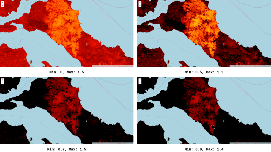
Visualization Caveat

This took a few tries to visualise correctly, which involved setting the maximum and minimum values to be displayed above. (i.e. what raw value of the index appears as white and what level appears as black, which in turn affects how the intensity of red changes throughout). As shown below, there were several color ranges tried, and this goes back to the application- and area- specific nature of any remote-sensing index.

Link to Google Collab

References

Fernández-Manso, A., Fernández-Manso, O., & Quintano, C. (2016). SENTINEL-2A red-edge spectral indices suitability for discriminating burn severity. International journal of applied earth observation and geoinformation, 50, 170-175.

Escuin, S., Navarro, R., & Fernandez, P. (2008). Fire severity assessment by using NBR (Normalized Burn Ratio) and NDVI (Normalized Difference Vegetation Index) derived from LANDSAT TM/ETM images. International Journal of Remote Sensing, 29(4), 1053-1073.

Cui Z, Kerekes JP. Potential of Red Edge Spectral Bands in Future Landsat Satellites on Agroecosystem Canopy Green Leaf Area Index Retrieval. Remote Sensing. 2018; 10(9):1458.