Modeling human/computer interactions on Star Trek 🖖

This is the latest in my series of screencasts demonstrating how to use the tidymodels packages, from just getting started to tuning more complex models. Today’s screencast is on a more advanced topic, how to evaluate multiple combinations of feature engineering and modeling approaches via workflowsets, with this week’s #TidyTuesday dataset on Star Trek human/computer interactions.

Here is the code I used in the video, for those who prefer reading instead of or in addition to video.

Explore data

Our modeling goal is to predict which computer interactions from Star Trek were spoken by a person and which were spoken by the computer.

library(tidyverse)
computer_raw <- read_csv("https://raw.githubusercontent.com/rfordatascience/tidytuesday/master/data/2021/2021-08-17/computer.csv")

computer_raw %>%
  distinct(value_id, .keep_all = TRUE) %>%
  count(char_type)


## # A tibble: 2 × 2
## char_type n
## <chr> <int>
## 1 Computer 178
## 2 Person 234

Which words are more likely to be spoken by a computer vs. by a person?

library(tidytext)
library(tidylo)

computer_counts <-
  computer_raw %>%
  distinct(value_id, .keep_all = TRUE) %>%
  unnest_tokens(word, interaction) %>%
  count(char_type, word, sort = TRUE)

computer_counts %>%
  bind_log_odds(char_type, word, n) %>%
  filter(n > 10) %>%
  group_by(char_type) %>%
  slice_max(log_odds_weighted, n = 10) %>%
  ungroup() %>%
  ggplot(aes(log_odds_weighted,
    fct_reorder(word, log_odds_weighted),
    fill = char_type
  )) +
  geom_col(alpha = 0.8, show.legend = FALSE) +
  facet_wrap(vars(char_type), scales = "free_y") +
  labs(y = NULL)

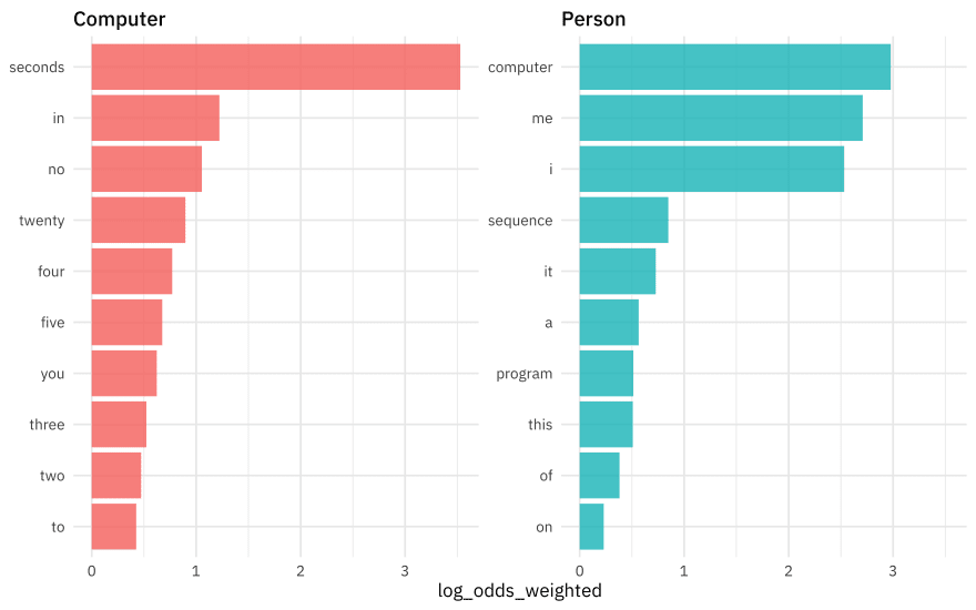
Notice that stop words are among the words with highest weighted log odds; they are very informative in this situation.

Build and compare models

Let’s start our modeling by setting up our “data budget.” This is a very small dataset so we won’t expect to see amazing results from our model, but it is fun and a nice way to demonstrate some of these concepts.

library(tidymodels)

set.seed(123)

comp_split <-
  computer_raw %>%
  distinct(value_id, .keep_all = TRUE) %>%
  select(char_type, interaction) %>%
  initial_split(prop = 0.8, strata = char_type)

comp_train <- training(comp_split)
comp_test <- testing(comp_split)

set.seed(234)
comp_folds <- bootstraps(comp_train, strata = char_type)
comp_folds


## # Bootstrap sampling using stratification 
## # A tibble: 25 × 2
## splits id         
## <list> <chr>      
## 1 <split [329/118]> Bootstrap01
## 2 <split [329/128]> Bootstrap02
## 3 <split [329/134]> Bootstrap03
## 4 <split [329/124]> Bootstrap04
## 5 <split [329/118]> Bootstrap05
## 6 <split [329/116]> Bootstrap06
## 7 <split [329/106]> Bootstrap07
## 8 <split [329/124]> Bootstrap08
## 9 <split [329/121]> Bootstrap09
## 10 <split [329/121]> Bootstrap10
## # … with 15 more rows

When it comes to feature engineering, we don’t know ahead of time if we should remove stop words, or center and scale the predictors, or balance the classes. Let’s create feature engineering recipes that do all of these things so we can compare how they perform.

library(textrecipes)
library(themis)

rec_all <-
  recipe(char_type ~ interaction, data = comp_train) %>%
  step_tokenize(interaction) %>%
  step_tokenfilter(interaction, max_tokens = 80) %>%
  step_tfidf(interaction)

rec_all_norm <-
  rec_all %>%
  step_normalize(all_predictors())

rec_all_smote <-
  rec_all_norm %>%
  step_smote(char_type)

## we can `prep()` just to check if it works
prep(rec_all_smote)


## Data Recipe
## 
## Inputs:
## 
## role #variables
## outcome 1
## predictor 1
## 
## Training data contained 329 data points and no missing data.
## 
## Operations:
## 
## Tokenization for interaction [trained]
## Text filtering for interaction [trained]
## Term frequency-inverse document frequency with interaction [trained]
## Centering and scaling for tfidf_interaction_a, ... [trained]
## SMOTE based on char_type [trained]

Now let’s do the same with removing stop words.

rec_stop <-
  recipe(char_type ~ interaction, data = comp_train) %>%
  step_tokenize(interaction) %>%
  step_stopwords(interaction) %>%
  step_tokenfilter(interaction, max_tokens = 80) %>%
  step_tfidf(interaction)

rec_stop_norm <-
  rec_stop %>%
  step_normalize(all_predictors())

rec_stop_smote <-
  rec_stop_norm %>%
  step_smote(char_type)

## again, let's check it
prep(rec_stop_smote)


## Data Recipe
## 
## Inputs:
## 
## role #variables
## outcome 1
## predictor 1
## 
## Training data contained 329 data points and no missing data.
## 
## Operations:
## 
## Tokenization for interaction [trained]
## Stop word removal for interaction [trained]
## Text filtering for interaction [trained]
## Term frequency-inverse document frequency with interaction [trained]
## Centering and scaling for 80 items [trained]
## SMOTE based on char_type [trained]

Let’s try out two kinds of models that often work well for text data, a support vector machine and a naive Bayes model.

library(discrim)

nb_spec <-
  naive_Bayes() %>%
  set_mode("classification") %>%
  set_engine("naivebayes")

nb_spec


## Naive Bayes Model Specification (classification)
## 
## Computational engine: naivebayes


svm_spec <-
  svm_linear() %>%
  set_mode("classification") %>%
  set_engine("LiblineaR")

svm_spec


## Linear Support Vector Machine Specification (classification)
## 
## Computational engine: LiblineaR

Now we can put all these together in a workflowset.

comp_models <-
  workflow_set(
    preproc = list(
      all = rec_all,
      all_norm = rec_all_norm,
      all_smote = rec_all_smote,
      stop = rec_stop,
      stop_norm = rec_stop_norm,
      stop_smote = rec_stop_smote
    ),
    models = list(nb = nb_spec, svm = svm_spec),
    cross = TRUE
  )

comp_models


## # A workflow set/tibble: 12 × 4
## wflow_id info option result    
## <chr> <list> <list> <list>    
## 1 all_nb <tibble [1 × 4]> <opts[0]> <list [0]>
## 2 all_svm <tibble [1 × 4]> <opts[0]> <list [0]>
## 3 all_norm_nb <tibble [1 × 4]> <opts[0]> <list [0]>
## 4 all_norm_svm <tibble [1 × 4]> <opts[0]> <list [0]>
## 5 all_smote_nb <tibble [1 × 4]> <opts[0]> <list [0]>
## 6 all_smote_svm <tibble [1 × 4]> <opts[0]> <list [0]>
## 7 stop_nb <tibble [1 × 4]> <opts[0]> <list [0]>
## 8 stop_svm <tibble [1 × 4]> <opts[0]> <list [0]>
## 9 stop_norm_nb <tibble [1 × 4]> <opts[0]> <list [0]>
## 10 stop_norm_svm <tibble [1 × 4]> <opts[0]> <list [0]>
## 11 stop_smote_nb <tibble [1 × 4]> <opts[0]> <list [0]>
## 12 stop_smote_svm <tibble [1 × 4]> <opts[0]> <list [0]>

None of these models have any tuning parameters, so next let’s use fit_resamples() to evaluate how each of these combinations of feature engineering recipes and model specifications performs, using our bootstrap resamples.

set.seed(123)
doParallel::registerDoParallel()

computer_rs <-
  comp_models %>%
  workflow_map(
    "fit_resamples",
    resamples = comp_folds,
    metrics = metric_set(accuracy, sensitivity, specificity)
  )

We can make a quick high-level visualization of these results.

autoplot(computer_rs)

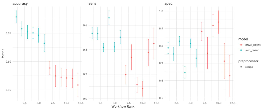
All of the SVMs did better than all of the naive Bayes models, at least as far as overall accuracy. We can also dig deeper and explore the results more.

rank_results(computer_rs) %>%
  filter(.metric == "accuracy")


## # A tibble: 12 × 9
## wflow_id .config .metric mean std_err n preprocessor model rank
## <chr> <chr> <chr> <dbl> <dbl> <int> <chr> <chr> <int>
## 1 all_svm Preprocess… accuracy 0.679 0.00655 25 recipe svm_l… 1
## 2 all_norm_… Preprocess… accuracy 0.658 0.00756 25 recipe svm_l… 2
## 3 stop_svm Preprocess… accuracy 0.652 0.00700 25 recipe svm_l… 3
## 4 all_smote… Preprocess… accuracy 0.650 0.00611 25 recipe svm_l… 4
## 5 stop_norm… Preprocess… accuracy 0.646 0.00753 25 recipe svm_l… 5
## 6 stop_smot… Preprocess… accuracy 0.632 0.00914 25 recipe svm_l… 6
## 7 all_norm_… Preprocess… accuracy 0.589 0.00678 25 recipe naive… 7
## 8 all_smote… Preprocess… accuracy 0.575 0.0115 25 recipe naive… 8
## 9 stop_smot… Preprocess… accuracy 0.573 0.00971 25 recipe naive… 9
## 10 stop_norm… Preprocess… accuracy 0.571 0.00950 25 recipe naive… 10
## 11 all_nb Preprocess… accuracy 0.570 0.0102 25 recipe naive… 11
## 12 stop_nb Preprocess… accuracy 0.559 0.0120 25 recipe naive… 12

Some interesting things to note are:

• how balancing the classes via SMOTE does in fact change sensitivity and specificity the way we would expect
• that removing stop words looks like mostly a bad idea!

Train and evaluate final model

Let’s say that we want to keep overall accuracy high, so we pick rec_all and svm_spec. We can use last_fit() to fit one time to all the training data and evalute one time on the testing data.

comp_wf <- workflow(rec_all, svm_spec)

comp_fitted <-
  last_fit(
    comp_wf,
    comp_split,
    metrics = metric_set(accuracy, sensitivity, specificity)
  )

comp_fitted


## # Resampling results
## # Manual resampling 
## # A tibble: 1 × 6
## splits id .metrics .notes .predictions .workflow
## <list> <chr> <list> <list> <list> <list>   
## 1 <split [329/83]> train/test split <tibble [… <tibble … <tibble [83 … <workflo…

How did that turn out?

collect_metrics(comp_fitted)


## # A tibble: 3 × 4
## .metric .estimator .estimate .config             
## <chr> <chr> <dbl> <chr>               
## 1 accuracy binary 0.735 Preprocessor1_Model1
## 2 sens binary 0.611 Preprocessor1_Model1
## 3 spec binary 0.830 Preprocessor1_Model1

We can also look at the predictions, and for example make a confusion matrix.

collect_predictions(comp_fitted) %>%
  conf_mat(char_type, .pred_class) %>%
  autoplot()

It was easier to identify people talking to computers than the other way around.

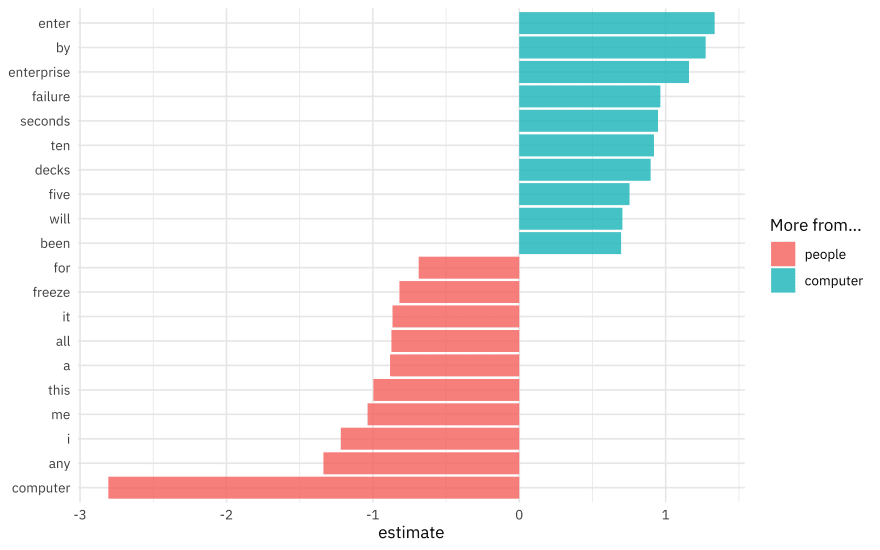
Since this is a linear model, we can also look at the coefficients for words in the model, perhaps for the largest effect size terms in each direction.

extract_workflow(comp_fitted) %>%
  tidy() %>%
  group_by(estimate > 0) %>%
  slice_max(abs(estimate), n = 10) %>%
  ungroup() %>%
  mutate(term = str_remove(term, "tfidf_interaction_")) %>%
  ggplot(aes(estimate, fct_reorder(term, estimate), fill = estimate > 0)) +
  geom_col(alpha = 0.8) +
  scale_fill_discrete(labels = c("people", "computer")) +
  labs(y = NULL, fill = "More from...")