
27 Min Read
The Story
In this post, I will walk you through how I built a deep learning network to identify and classifier 102 different types of flowers using Pytorch library.
The purpose of this post is to help others like me, who were eager and curious to learn AI/Machine Learning but did not know where to start.
Before we get started we need to look at the data we are working with, as well as how the folder structure is set up for this project. The folder structure used in this situation is how you should set up your folders for essentially every PyTorch model you create.
Depending on the type of project and amount of data, you will want either two groups:
- Train
- Test
Or you may want three groups:
- Train
- Validation
- Test
In my case, I had my data directories in the manner shown below.
$ ls flower/test/ | wc -l
102

$ ls flower/train |wc -l
63

$ ls flower/valid |wc -l
102

$ tree flowers -L 3

flowers
├── test
│   ├── 1
│   │   ├── image_06743.jpg
│   │   └── image_06764.jpg
│   ├── 102
│   │   ├── image_08004.jpg
│   │   ├── image_08012.jpg
│   │   ├── image_08015.jpg
│   │   ├── image_08023.jpg
│   │   ├── image_08030.jpg
│   │   └── image_08042.jpg
├── train
│   ├── 1
│   │   ├── image_07086.jpg
│   │   ├── image_07087.jpg
│   ├── 102
│   │   ├── image_08000.jpg
│   │   ├── image_08001.jpg
│   │   ├── image_08003.jpg
└── valid
    ├── 1
    │   ├── image_06739.jpg
    │   ├── image_06749.jpg
    │   ├── image_06755.jpg
    ├── 102
    │   ├── image_07895.jpg
    │   ├── image_07904.jpg
    │   ├── image_07905.jpg

270 directories, 5715 files
Within each directory, you will want a separate folder for each class. In the case of the project, this meant a separate folder for each of the 102 flower classes. Each flower was labelled as a number.
For each of the flower types, the training dataset had between 27-206 images, the validation dataset had between 1-28 images, and the testing dataset had between 2-28 images.
Original images were obtained from the 102 Category Flower Dataset, and they are described in the following way by the authors Maria-Elena Nilsback and Andrew Zisserman
Flowers categories can be found here
The Walk-through
In this section, I will detail a step-by-step on how I built an AI-based flower classifier using Pytorch. I trained an image classifier to recognize different species of flowers. In machine learning, this is called supervised learning (we want to map an input to output labels).
A typical application would be using something like this in as a phone app that tells you the name of the flower (or just about any image) your camera is looking at.

This step-by-step assumes you have some knowledge of Python and will not go into the details as to know to install it and the modules used.
Package Imports
All the necessary packages and modules are imported in the first cell of the notebook.
import json
import time

from collections import OrderedDict
from datetime import datetime
from pathlib import Path

# A Tensor library like NumPy, with strong GPU support
import torch  # version 0.4.0

from matplotlib import pyplot as plt

# A neural networks library deeply integrated with autograd designed for maximum flexibility.
from torch import nn
from torch import optim
# DataLoader and other utility functions for convenience
from torch.utils.data import DataLoader

# Transforms are used to augment the training data with random scaling, rotations, mirroring, and/or cropping.
from torchvision import datasets, models, transforms
Training data augmentation
The dataset is split into three parts, training, validation, and testing.
For the training, I needed to apply image transformations such as random scaling (224x224 pixels as required by the pre-trained network), cropping and flipping. This helped the network generalize leading to better performance.
The validation and testing sets are used to measure the model's performance on data it hasn't seen yet. I needed to resize and crop the images to the appropriate size.
The pre-trained networks I used were trained on the ImageNet dataset where each colour channel was normalized separately. For all three sets, I needed to normalize the means and standard deviations of the images to what the network expects. For the means, it's [0.485, 0.456, 0.406] and for the standard deviations [0.229, 0.224, 0.225], calculated from the ImageNet images. These values will shift each colour channel to be centred at 0 and range from -1 to 1.
data_dir = 'flowers'
train_dir = data_dir + '/train'
valid_dir = data_dir + '/valid'
test_dir = data_dir + '/test'

_img_size = 224
_orig_img_size = 256
_mean = [0.485, 0.456, 0.406]
_std_dev = [0.229, 0.224, 0.225]

# `transforms.Compose` lets you compose multiple transforms together so we can use more than one transformation.
train_transforms = transforms.Compose([
    transforms.RandomRotation(30),
    transforms.RandomResizedCrop(_img_size), # Randomly resized and cropped images to 224x224
    transforms.RandomVerticalFlip(),
    transforms.ToTensor(),  # Convert to a tensor
    transforms.Normalize(   # Normalize
        _mean,  # Means
        _std_dev,  # Standard deviation
    )
])

valid_transforms = transforms.Compose([
    transforms.Resize(_orig_img_size),
    transforms.CenterCrop(_img_size),
    transforms.ToTensor(),  # Convert to a tensor
    transforms.Normalize(   # Normalize
        _mean,  # Means
        _std_dev,  # Standard deviation
    )
])

test_transforms = transforms.Compose([
    transforms.Resize(_orig_img_size),
    transforms.CenterCrop(_img_size),
    transforms.ToTensor(),  # Convert to a tensor
    transforms.Normalize(   # Normalize
        _mean,  # Means
        _std_dev,  # Standard deviation
    )
])

# Using `ImageFolder` and `DataLoader` allows for the ability to easily pass the images through the necessary transformations and then through our network for training or prediction.
train_datasets = datasets.ImageFolder(train_dir, transform=train_transforms)
valid_datasets = datasets.ImageFolder(valid_dir, transform=valid_transforms)
test_datasets = datasets.ImageFolder(test_dir, transform=test_transforms)

train_loaders = DataLoader(train_datasets, batch_size=32, shuffle=True)
valid_loaders = DataLoader(valid_datasets, batch_size=32, shuffle=True)
test_loaders = DataLoader(test_datasets, batch_size=32, shuffle=True)
I also need to load in mapping from category label to category name of the flowers. This file contained a dictionary mapping the integer encoded categories to the actual names of the flowers.
with open('cat_to_name.json', 'r') as f:
    cat_to_name = json.load(f)
print(len(cat_to_name))
Building and training the classifier
Now that the data is ready, it's time to build and train the classifier. When training I had to ensure that I was only updating the weights of the feed-forward network as I was using a pre-trained model.
Image recognition models have two parts:
- The Convolutional part and, [Freeze]
- The Classifier part [Train]
We want to keep the pre-trained convolutional part but put in our classifier. Here’s why:
The convolution/pooling section of our model is used to recognize the features inside an image. It first identifies edges, then using the edges it identifies shapes, and using the shapes it can identify objects. But it takes A LOT of data and time to train this section hence why we freeze this section instead. These pre-trained convolutional layers were trained to identify these feature very well, regardless of what kind of image you have.
The last part of the model is the classifier. The classifier takes all the information extracted from the photo in the convolution part and uses it to identify the image. This is the part of the pre-trained model we want to replace and to train on our images. This makes the model tailored to identify the images we give it.
I used one of the pre-trained models from torchvision.models to get the image features. There's quite a library of different models to download. I chose a model called densenet161 and specified that we want it to be pre-trained by setting pretrained=True.
Then, we want to make sure we don’t train this model since it is already trained, and we only want to train the classifier we will put in next. We tell the model not to calculate the gradients of any parameter since that is only done for training.
# Load a pre-trained network using `torchvision.models` library
model = models.densenet161(pretrained=True)
model.arch = model.__name__ = model.__module__.split('.')[-1]

print(f"{model.arch.title()!r} model Before classifier update: \n>> {model.classifier}")

def new_classifier(model):
    """Define a new, untrained feed-forward network as a classifier, using
    ReLU activations and dropout.
    """
    # This ensures that the convolutional layer does not get trained.
    for param in model.parameters():
        param.requires_grad = False

    # To update existing classifier one, has to ensure that the number
    # of inputs matches the number of outputs from the convolutional section/
    # layer.
    in_features = (
        model.classifier.in_features
        if hasattr(model.classifier, "in_features")
        else model.classifier[0].in_features
    )
    out_features = (
        1000
        if hasattr(model.classifier, "out_features")
        else model.classifier[0].out_features
    )

    new_classifier = nn.Sequential(OrderedDict([
            ("drop_out", nn.Dropout(p=0.5)),
            ("fc1", nn.Linear(in_features, out_features)),
            ("relu", nn.ReLU(inplace=True)),
            ("drop_out", nn.Dropout(p=0.5)),
            ("relu", nn.ReLU()),
            # In order to determine the number of outputs. We calculated the
            # number of categories in the flower labels file. The model will
            # output a list of probabilities, each corresponding to how
            # certain the picture is to that label.
            ("fc2", nn.Linear(out_features, len(cat_to_name))),
            # Activation functions helps the model learn complex relationships
            # between the input and the output. We use ReLU on all layers
            # except for the output.
            ("relu", nn.ReLU()),
            ("output", nn.LogSoftmax(dim=1)),
            # The Softmax function turns the outputted numbers into
            # probabilities for each label.
            ])
    )
    return new_classifier
Having defined the new_classifier we need to replace the default classifier of the model with our classifier. Classifiers are fully connected neural networks, so to do this, we must first build our neural network.
A neural network is just a method to find complex patterns and connections between numbers of the input and the output. In this case, it takes the features of the image that were highlighted by the convolution section to determine how likely the image is a certain label.
model.classifier = new_classifier(model)
Now the model is created! Next, we just need to train it.
Training the network
Training a model requires a lot of computational resources which then means that training a model on a GPU is much faster than training a CPU. However, GPU computing does not come cheap and in most cases GPU's are not available. But that does not stop one from trying to use the GPU for computation. We use Torch to check which device is available for you. If there is a compatible GPU, we set the variable to GPU, if not, it sticks with CPU. We then move our model to this device.
device = torch.device("cuda:0" if torch.cuda.is_available() else "cpu")
model.to(device)
print(f"Model using the {device} device for training.")
While training, we need to determine how inaccurate our model is. To evaluate the amount of error our model has, we use nn.NLLLoss. This function takes in the output of our model, for which we used the nn.LogSoftmax function.
To train our model, we take our error and see how we can adjust the weights we multiplied our numbers by to get the smallest error. The method of calculating how we adjust our weights and applying it to our weights is called Adam (On linear problems we would use Gradient Descent). PyTorch has a torch.optim package with various optimization algorithms like SGD (Stochastic Gradient Descent), Adam, RMSprop etc.
Optimizers are used to update weights and biases i.e. the internal parameters of a model to reduce the error.
learning_rate = 0.001  # Rate at which the model learns
criterion = nn.NLLLoss()
optimizer = optim.Adam(params=model.classifier.parameters(), lr=learning_rate)
Now that we are all set we can begin training out model. To ensure that the model goes through the entire data set we use a for loop. Every time it has gone over the entire set of images, it is called an epoch. In one epoch we want the model to go through both the training set and the validation set, but the model into training mode model.train() and move the model and data to GPU model.to(device). The optimizer.zero_grad() ensures that the weights/gradients are zeroed/cleared before parsing the data to the model.forward() in order to calculate our output.
We then calculate the adjustments we need to decreases this error by calling loss.backward() and use our optimizer to adjust the weights by calling optimizer.step().
As we train, we want to know how things are going, so we keep track of the total errors we calculated and print out the progress of the training.
def train(epochs=2, print_every=40):
    steps = 0
    running_loss = 0
    for epoch in range(epochs):
        model.train()
        running_loss = 0
        for images, labels in iter(train_loaders):
            images, labels = images.to(device), labels.to(device)
            steps += 1

            optimizer.zero_grad()
            # Forward pass
            output = model.forward(images)

            loss = criterion(output, labels)
            # Calculate the gradient through back-propagation
            loss.backward()
            # Adjust parameters based on gradients
            optimizer.step()
            # Add the loss to the training set's running loss
            running_loss += loss.item()

            if steps % print_every == 0:
                # Put model in evaluation/testing mode
                model.eval()
                # Do not calculate gradients
                with torch.no_grad():
                    validation_loss, validation_accuracy = validation(
                        model, valid_loaders, criterion
                    )

                print(
                    f"Timestamp: {datetime.now()}.."
                    f"Model: {model.arch}.."
                    f"Epoch: {epoch + 1} / {epochs}.."
                    f"Training Loss: {running_loss / print_every:.3f}%.."
                    f"Validation Loss: {validation_loss / len(valid_loaders):.3f}%.."
                    f"Validation Accuracy: {validation_accuracy / len(valid_loaders) * 100:.3f}%.."
                )
                running_loss = 0
                # Done evaluating now return model back to training.
                model.train()

train()
To ensure that our model is being properly trained we to run it through the validation stage where we evaluate a piece of the trained model. By setting our model to evaluation mode model.eval() and iterating over all the images(validation) in our set we can calculate how accurate it is.
Our model used the LogSoftmax function to increase computation speed, but humans prefer simple and readable statistics thus we convert the output to real percentages. We use use torch.exp to reverse the log function. We now want to evaluate if our model's prediction is correct by calculating the average accuracy by comparing the labels.data which the maximum value the model predicted.
After going through both the training and validation set, we want to print the errors for both and the accuracy of the validation set.
def validation(model, validloader, criterion):
    test_loss = 0
    accuracy = 0
    for images, labels in validloader:
        images, labels = images.to(device), labels.to(device)

        output = model.forward(images)
        test_loss += criterion(output, labels).item()
        # Calculate the probability
        probability = torch.exp(output)
        equality = (labels.data == probability.max(dim=1)[1])
        accuracy += equality.type(torch.FloatTensor).mean()
    return test_loss, accuracy
If everything is set up correctly, you should see something like the following:
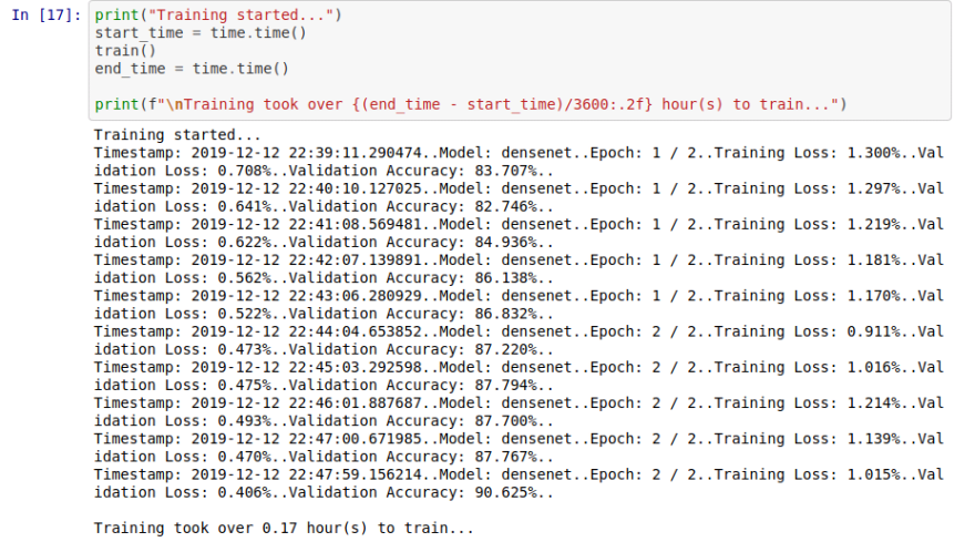
The densenet161 pre-trained model appears to be learning with each epoch, having an accuracy of 90% in under 20 minutes on training using a GPU and it doesn’t appear that our model is over-fitting.
I found that by increasing the number of epochs or decreasing the learning rate this would improve the accuracy of my model but can also be expensive to compute.
Model Evaluation
For a sanity check, one has test the new classifier model against the testing dataset images just to confirm whether the model does what it should or not. I used some most of the validation code to create a test_model function which computes the accuracy of the model.
You will notice a few changes from earlier:
- By using
torch.no_grad(), it simply means I am not interested in training with this function. - To get the output, I need to complete a single forward pass of our testing data (image) using
model.forward(images). Note that the output is a tensor (think of a tensor as a multidimensional array) with one dimension of 102 values for the LogSoftmax output values from the model for each image prediction, and another dimension of 32 values for each of the images in the batch. - Then using the
maxmethod to get the maximum probability value, we can get the most likely image. Specifically, you obtain the maxLogSoftmaxvalue for each image and the predicted image label (stored in predicted). - Then we can look at if the predicted label matches the actual data label.
- The
equalitytensor holds a value between 0 and 1, a value closer to 1 means the prediction is correct, and a value closer to 0 means the prediction is incorrect.
def test_model(model, test_loaders, _threshold=70):
    accuracy = 0
    model.eval()
    model.to(device)

    for images, labels in iter(test_loaders):
        images, labels = images.to(device), labels.to(device)

        with torch.no_grad():
            output = model.forward(images)
            probability = torch.exp(output)
            equality = (labels.data == probability.max(dim=1)[1])
            accuracy += equality.type(torch.FloatTensor).mean()

    _model_acc =  (accuracy / len(test_loaders)) * 100
    return (
        f"Model failed to meet minimum accuracy of {_threshold}%"
        if _model_acc <= _threshold
        else _model_acc
    )
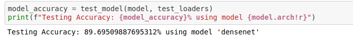
From the image below one can easily see that the accuracy of the prediction is just over 89%, which simply means that our model is doing exactly what it's supposed to do.
Finally using the model
After confidently building a model with an accuracy of 89% we can now complete the image classifier. The idea is to give it random images and predict what image it is.
Lets randomly select an image from the dataset and parse it through our model to predict if the model with accurately guess what the flower is. From the flower category we know that the flower is a hibiscus'

Processing Images
Now we will read the image using PIL image library and feed it into our transformation pipeline for necessary preprocessing and later use the model for prediction. The processing includes scaling/resizing/normalizing the image the same way we scaled the test and validation images earlier in the project and converting it into a numpy array.
def process_image(image_path, size=(256, 256), crop_size=244):
    """
    Scales, crops, and normalizes a PIL image for a PyTorch model, returns an Numpy array
    """
    image_path = Path(image_path)
    if not Path(image_path).is_file():
        raise RuntimeError(
            f"Image file {image_path.as_posix()!r} doesn't exist."
        )
    # Load the image
    image = Image.open(image_path)
    # https://pillow.readthedocs.io/en/latest/reference/Image.html#PIL.Image.Image.resize
    image = image.resize(size, Image.ANTIALIAS)
    assert image.size == size, f"Image resized to {image.size}, instead of {size}"
    h, w = size
    dim = {
        "left": (w - crop_size) / 2,
        "lower": (h - crop_size) / 2,
        "right": ((w - crop_size) / 2) + crop_size,
        "top": ((h - crop_size) / 2) + crop_size,
    }

    cropped_image = image.crop(tuple(dim.values()))
    assert cropped_image.size == (
        crop_size,
        crop_size,
    ), f"Image resized to {cropped_image.size}, instead of {crop_size}"

    # make image values to be 1's and 0's
    image_array = np.array(cropped_image) / (size[0] - 1)
    image_array = (image_array - np.array(MEAN)) / np.array(STD_DEV)
    # Make the color channel dimension first instead of last
    image_array = image_array.transpose((2, 0, 1))
    assert isinstance(image_array, np.ndarray)
    return image_array
Class Prediction
Once I got the images in the correct format, it was time to write a function for making predictions with my model. A common practice is to predict the top 5 or so (usually called top-K) most probable classes. I had to calculate the class probabilities to find the K largest values.
To get the top K largest values in a tensor I used x.topk(k). This method returns both the highest k probabilities and the indices of those probabilities corresponding to the classes. I had to convert from these indices to the actual class labels using class_to_idx which I added to the model. I had to switch the direction of the keys and values such that I could index using what was provided back from the model to pull the class number.
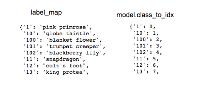
image label_map: class -> flower, class_to_idx: class -> pred
def predict(image, model, gpu=False, topk=5):
    """Predict the class (or classes) of an image using a trained deep learning model."""
    try:
        assert isinstance(
            image, np.ndarray
        ), "Image is not a numpy array, will process image into an array."
    except AssertionError:
        image = process_image(image)

    model.eval()
    device = model.device
    model.to(device)

    # RuntimeError: Input type (torch.cuda.DoubleTensor) and weight type
    # (torch.cuda.FloatTensor) should be the same

    # Convert a Numpy array into a Tensor
    img = (
        torch.from_numpy(image).type(torch.cuda.FloatTensor)
        if gpu
        else torch.from_numpy(image).type(torch.FloatTensor)
    )
    # https://discuss.pytorch.org/t/expected-stride-to-be-a-single-integer-value-or-a-list/17612
    img = img.unsqueeze(0)
    img.to(device)
    img = Variable(img).to(device)

    output = model.forward(img)
    probabilities = torch.exp(output)
    probs, indices = probabilities.topk(topk)

    # Convert cuda tensor to numpy array then to list.
    def tensor_to_list(l):
        return l.to("cpu").detach().numpy().tolist()

    # Convert nested list into a list
    def flatten(l):
        return [item for sublist in l for item in sublist]

    probs = tensor_to_list(probs)
    indices = tensor_to_list(indices)

    probs = (
        flatten(probs)
        if any(isinstance(i, list) for i in probs)
        else probs
    )
    indices = (
        flatten(indices)
        if any(isinstance(i, list) for i in indices)
        else indices
    )

    class_to_idx = model.class_to_idx
    # Flip values with keys, to index easily.
    idx_to_class = dict(zip(class_to_idx.values(), class_to_idx.keys()))
    classes = [idx_to_class[idx] for idx in indices]

    return probs, classes
Sanity Check
The last part of the project was basically to glue up the functions shown above for processing the image and predicting the label into a simple sanity_check function that expects the path to an image, the trained model and the labels.
def sanity_check(image_path, model, labels):
    """Checks if the prediction matched the correct flower name."""
    if not isinstance(image_path, Path):
        image_path = Path(image_path)

    image = process_image(image_path)
    probs, classes = predict(image, model)

    fig = plt.figure(figsize=(5,10))
    ax1 = fig.add_subplot(211)
    ax1.axis('off')
    ax2 = fig.add_subplot(212)
    plt.subplots_adjust(wspace = 0.5)

    # By converting from the class integer encoding to actual flower
    # names with the `cat_to_name.json` file that contains labels from
    # earlier we can show a PyTorch tensor as an image together with
    # it's predicted output
    predicted_flower = labels[image_path.parent.name]
    other_flowers = [labels[x] for x in classes]
    imshow(image, ax=ax1, title=predicted_flower.title())
    ax2.barh(other_flowers, probs, 0.5)


sanity_check(image_path, model, cat_to_name)
The function uses the trained model for predictions, and we need to ensure that it makes sense. Even if the testing accuracy is high, it's always good to check that there aren't obvious bugs. By using matplotlib library I was able to plot the probabilities for the top 5 classes as a bar graph, along with the input image. The prediction is shown below.

Upon completion I uploaded my code and a day later after reviewing, I was greeted with the message below:

This concludes the walk-through and the Jupyter notebook and Python scripts can be found on my GitHub learning-progress repository
I would encourage you to create your image classifier using this template: AI Programming with Python Project
Resources
I personally found this talk by @stefanotte titled: Deep Neural Networks with PyTorch very helpful in understanding concepts.
This Pytorch tutorial by @Sentdex on Deep Learning and Neural Networks with Python and Pytorch p.1 was interesting.
Other useful resources.
- Transfer Learning with Pytorch
- Pytorch Tutorials
- Training AlexNet with tips and checks on how to train CNNs: Practical CNNs in PyTorch
- Get Started with PyTorch – Learn How to Build Quick & Accurate Neural Networks
- Transfer Learning with Convolutional Neural Networks in PyTorch
- PyTorch for Deep Learning: A Quick Guide for Starters
- Recommended Free Course: Practical Deep Learning for Coders, v3

Top comments (0)