Sometimes we want to highlight the rows if any cell in that row contains a specific text or value in Excel. For achieving this you can use the conditional formatting option. This article provides some simple formulas to help you quickly get it done. Let’s see them below!! Get an official version of ** MS Excel** from the following link: https://www.microsoft.com/en-in/microsoft-365/excel
General Formula:
- You can use the below formula to highlight the entire row that meets a certain condition.
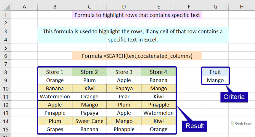
=SEARCH(text,cocatenated_columns)
Syntax Explanations:
- SEARCH – The SEARCH function helps to locate the character between two text strings and returns to the number of the starting position of the first text string from the first character of the second text string.
- Text – It specifies the criteria value that you want to highlight.
- Concatenated_columns – It represents all the column values from the same row.
- Comma symbol (,) – It is a separator that helps to separate a list of values.
- Parenthesis () – The main purpose of this symbol is to group the elements.
Practical Example:
Let’s consider the below example image.
- First, we will enter the input values in Column B to Column E.
- Now we want to highlight the entire row if any cell of that row contains the specific text which is given in Column G.

- So apply the above-given formula in the conditional formatting option.
- To know how to apply conditional formatting in Excel, just refer to this article: How to Apply the Formula with Conditional Formatting In Excel?
- Finally, it will highlight the result and displayed it as shown below.

Wrap-Up:
From this short tutorial, we have discussed the simple formula used to highlight the rows that contain specific text in Excel. If you have any doubts or queries mention them in the comment box below. Thank you. Click here to know more about Geek Excel *and Excel Formulas *!!

Top comments (0)