One of the things I like about R is how easy it is to create a visualization using ggplot2. This is great for exploratory data analysis. Instead of struggling with the data visualization library, you can focus on understanding data and relationships.
Plotnine is a Python library that is trying to solve this problem. It implements grammar of graphics and is based on ggplot2. For you who do not know, the grammar of graphics is a plotting framework introduced by Leland Wilkinson back in 1999. It consists of distinct layers of grammatical elements and meaningful plots through aesthetic mapping. The grammatical elements include, among others, data, aesthetics, geometries, and statistics. Plotting with grammar is powerful, and it makes the plot easy to think about and create.
To help me understand the Plotnine library better, I will explore the library by creating several plots in this article. I have included the code so you can create the plot yourself.
Scatter plot
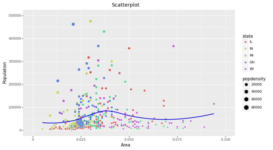
A Scatter plot is probably the most frequently used plot for data analysis, and it is used to show the relationships between two variables. In Plotnine, you can draw this using geom_point(). In the following plot, I have added geom_smooth, which draws a smoothing line.
from plotnine import *
from plotnine.data import midwest

(ggplot(midwest, aes(x="area", y="poptotal"))
 + geom_point(aes(color="state", size="popdensity"), na_rm=True)
 + geom_smooth(method="loess", color="blue", alpha=0.1, se=False)
 + xlim((0, 0.1))
 + ylim((0, 500000))
 + labs(title="Scatterplot",
        y="Population",
        x="Area")
 + theme(figure_size=(10, 6))
)
Jittered Plot
When we are drawing a lot of data points, chances are there will be many overlapping points appearing as a single dot. There are several ways to solve this issue. For instance, we can add transparency or use a hollow shape. Another way to solve this problem is to use geom_jitter. This randomly jittered the data points around their original position based on a threshold controlled by the width argument.
from plotnine import *
from plotnine.data import mpg

(ggplot(mpg, aes(x="cty", y="hwy"))
 + geom_jitter(width=0.5, size=1)
 + geom_smooth(method="lm", color="blue", se=False)
 + labs(y="hwy",
        x="cty",
        title="Jittered Points")
 + theme_bw()
 + theme(figure_size=(10, 6))
)
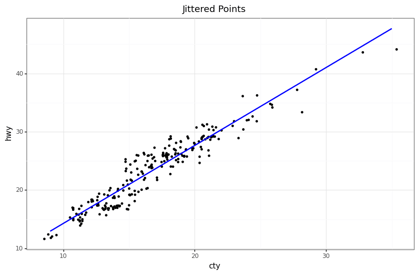
One downside of jittering is that it changes the data, so you must use it with care. If we jitter too much, we end up placing the points that do not represent the dataset.
Count Chart
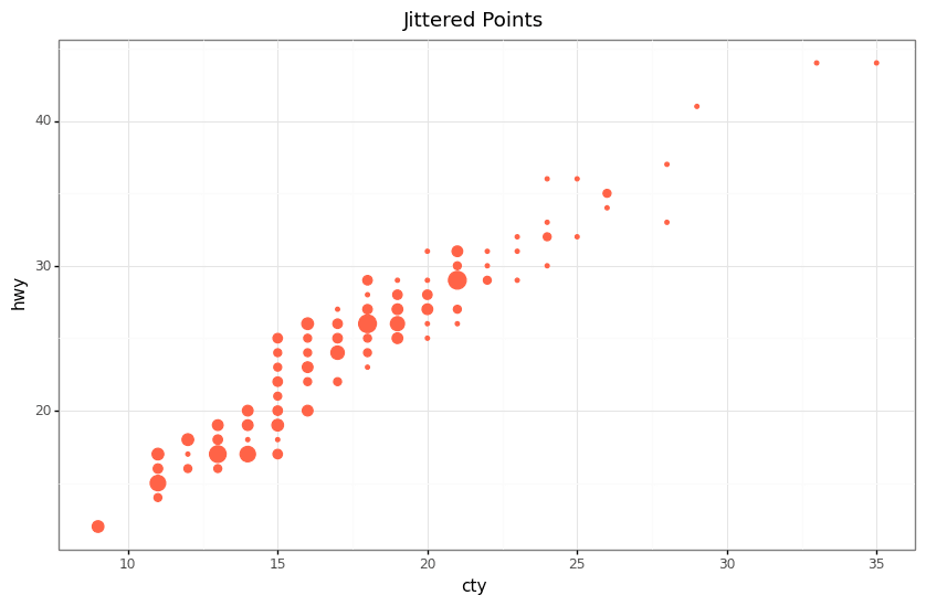
Another option to overcome overlapping data points is to use count charts. In a count chart, the size of the data point gets more prominent as more points overlap.
from plotnine import *
from plotnine.data import mpg

(ggplot(mpg, aes(x="cty", y="hwy"))
 + geom_count(color="tomato", show_legend=False)
 + labs(title="Jittered Points",
        x="cty",
        y="hwy")
 + theme_bw()
 + theme(figure_size=(10, 6))
)
Diverging bars
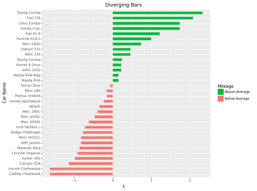
Sometimes we want to have a visualization that compares and contrasts data. There are several ways we can achieve this. But we will use geometry to highlight differences for this one.
In the plot below, we will use diverging bars to highlight differences. We will show which cars mpg that is above or below average and contrast them. To achieve this, we first need to make a new variable mpg_z that stores the car’s z score.
import numpy as np
from plotnine import *
from plotnine.data import mtcars

mtcars_df = (mtcars
             .assign(mpg_z=lambda x: round((x.mpg - np.mean(x.mpg))/np.std(x.mpg), 2))
             .assign(mpg_type=lambda x: np.where(x.mpg_z < 0, "below", "above"))
            )

(ggplot(mtcars_df, aes(x="reorder(name, mpg_z)", y="mpg_z"))
 + geom_bar(stat="identity", mapping=aes(fill="mpg_type"), width=.5)
 + scale_fill_manual(name="Mileage",
                     labels = ["Above Average", "Below Average"],
                     values = {"above":"#00ba38", "below":"#f8766d"})
 + coord_flip()
 + labs(y = "z", x = "Car Name", title= "Diverging Bars")
 + theme(figure_size=(8, 8))
)
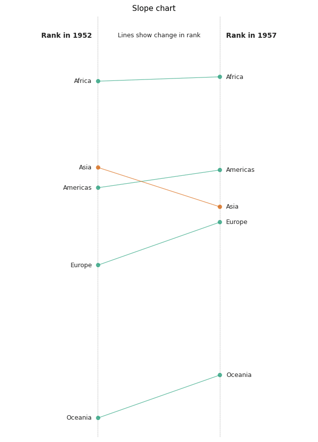
Slope chart
Another way to compare and contrast between two instances is to use a slope chart. Slope charts are simple graphs that show changes or rankings. Using a slope chart, you can quickly know what has gone up or down or remained the same. To create this plot, we utilize geom_point and geom_segment.
import pandas as pd

url = "https://raw.githubusercontent.com/selva86/datasets/master/gdppercap.csv"
df = pd.read_csv(url)
df = df.assign(gdp_diff_class=lambda x: np.where(x['1957'] - x['1952'] < 0, "red", "green"))

(ggplot(df)
 + geom_text(aes(2, '1952', label='continent'), nudge_x=0.05, ha='left', size=9, color="#252525")
 + geom_text(aes(1, '1957', label='continent'), nudge_x=-0.05, ha='right', size=9, color="#252525")
 + geom_point(aes(2, '1952', color='gdp_diff_class'), size=2.5, alpha=.7)
 + geom_point(aes(1, '1957', color='gdp_diff_class'), size=2.5, alpha=.7)
 + geom_segment(aes(x=2, y='1952', xend=1, yend='1957', color='gdp_diff_class'), alpha=.7, show_legend=False)
 + geom_vline(xintercept=1, linetype="dashed", size=.1)
 + geom_vline(xintercept=2, linetype="dashed", size=.1)
 + annotate('text', x=1, y=0, label='Rank in 1952', fontweight='bold', nudge_x=-0.05, ha='right', size=10, color="#222222")
 + annotate('text', x=2, y=0, label='Rank in 1957', fontweight='bold', nudge_x=0.05, ha='left', size=10, color="#222222")
 + annotate('text', x=1.5, y=0, label='Lines show change in rank', size=9, color="#252525")
 + labs(title="Slope chart")
 + lims(x=(0.35, 2.65))
 + scale_y_reverse()
 + scale_color_brewer(type='qual', palette=2, guide=False)
 + theme_void()
 + theme(figure_size=(8, 11))
)
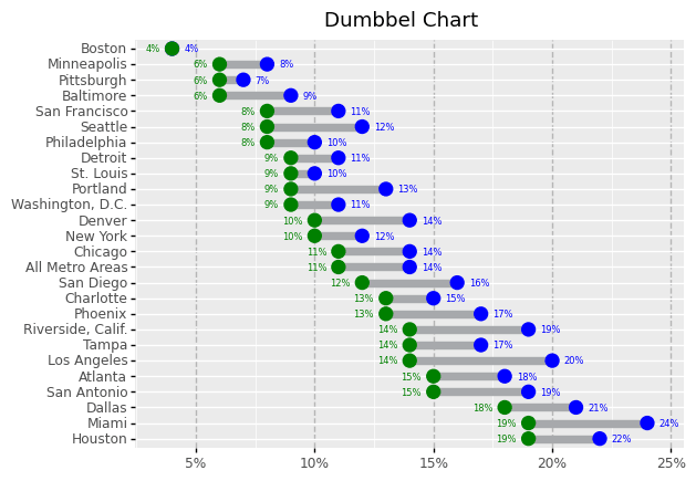
Dumbell plot
Dumbbell plot are typically used if you want to visualize relative positions (like growth and decline) between two points in time. You can also use it to compare distance between two categories. In the following plot we show a dumbell chart using geom_point and geom_smooth.
import pandas as pd

url = "https://raw.githubusercontent.com/selva86/datasets/master/health.csv"
health_df = pd.read_csv(url)
health_df["Area"] = pd.Categorical(health_df["Area"], categories=health_df["Area"])

def percentage_formatter(props):
    fmt = '{:.0f}%'.format
    return [fmt(p * 100) for p in props]

(ggplot(health_df)
 + geom_segment(aes(x='pct_2013', xend='pct_2014', y="Area", yend="Area"), color="#a7a9ac", size=3)
 + geom_point(aes(x='pct_2013', y='Area'), color="blue", size=4, stroke=0.7)
 + geom_point(aes(x='pct_2014', y='Area'), color="green", size=4, stroke=0.7)
 + geom_text(aes(x="pct_2013", y="Area", label="percentage_formatter(pct_2013)"), size=6, nudge_x=0.005, ha="left", color="blue")
 + geom_text(aes(x="pct_2014", y="Area", label="percentage_formatter(pct_2014)"), size=6, nudge_x=-0.005, ha="right", color="green")
 + scale_x_continuous(labels=lambda l: ["%d%%" % (v * 100) for v in l])
 + labs(title="Dumbbel Chart", x="", y="")
 + theme(panel_grid_major_x=element_line(linetype='dashed', color="gray", alpha=0.5))
)
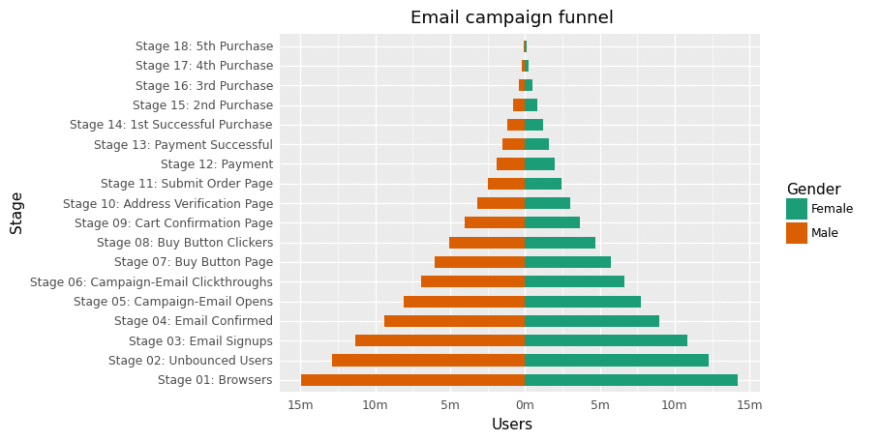
Population Pyramid
Population pyramids show how much population or what percentage of the population falls under a particular category. Population Pyramids are ideal for detecting changes or differences in population patterns. In this example, we show how males or females responded to an email campaign.
import pandas as pd

url = "https://raw.githubusercontent.com/selva86/datasets/master/email_campaign_funnel.csv"
email_campaign_funnel = pd.read_csv(url)

breaks = list(range(-15000000, 15000001, 5000000))
labels = ['{}m'.format(i) for i in range(15, 0, -5)] + ['{}m'.format(i) for i in range(0, 16, 5)]

(ggplot(email_campaign_funnel, aes(x="Stage", y="Users", fill="Gender"))
 + geom_bar(stat="identity", width=0.6)
 + scale_y_continuous(breaks=breaks, labels=labels)
 + coord_flip()
 + labs(title="Email campaign funnel")
 + scale_fill_brewer(type="qual", palette="Dark2")
 + theme(plot_title=element_text(hjust=0.5), axis_ticks=element_blank())
)
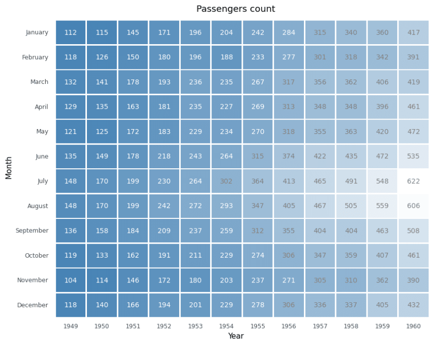
Heatmap
Heatmap map data values into colors. Heatmap is a great tool to show variation visually over time rather than the actual value itself, and it does an excellent job of highlighting broader trends. In this plot, we visualize the number of passengers count from 1949 to 1960 and highlight the trends over those years.
import numpy as np
import pandas as pd

url = "https://raw.githubusercontent.com/mwaskom/seaborn-data/master/flights.csv"
flights = pd.read_csv(url)

months = flights['month'].unique()
flights['month'] = pd.Categorical(flights['month'], categories=months)

text_color = flights.assign(text_color=lambda x: np.where(x.passengers < 300, "white", "grey"))['text_color']

(ggplot(flights, aes('factor(year)', 'month', fill='passengers'))
 + geom_tile(aes(width=.95, height=.95))
 + geom_text(aes(label='passengers'), size=10, color=text_color)
 + scale_y_discrete(limits=months[::-1])
 + scale_fill_gradient(low="steelblue", high="white")
 + labs(title="Passengers count", x="Year", y="Month")
 + theme(
     axis_ticks=element_blank(),
     panel_background=element_rect(fill='white'),
     legend_position="none",
     figure_size=(10, 8))
)
Summary
From this short preview of the library, I think Plotnine library is fantastic. It is still not as complete as ggplot2. For example, you can not add a caption or subtitle to a plot. And then in ggplot2 you have all this vast additional library that you can use to make even more plots (parallel sets, dendrograms, etc.) which is not available on the Python side yet. Overall, it is a great library to use, and I think this should be the standard for doing exploratory data analysis in Python.

Latest comments (0)