
Table of Contents
- Introduction
- Disclaimer
- Getting started
- Coding
- Conclusion
- References
Introduction
Hey there! So, I've been wanting to get into machine learning, and what better way to learn than to dive right in and start talking about it? As Frank Oppenheimer said, "The best way to learn is to teach.". Even though I might not be at a level to teach anyone yet 🤪.
Now, I know many of you might be familiar with k-NN in machine learning, but I thought, why not take a different route? Let's roll up our sleeves and create a k-NN model using good old C++—from scratch, focusing on identifying Iris types. No library, just plain coding. Well, this will help us understand what the heck is going on under the hood, without relying too much on the magic Python. Doing this will help you appreciate what Python does for us without us realizing it.
Disclaimer
I'm very new to machine learning and C++ stuff, so there might be a mistake in my code or in my explanation, and this is also my first time writing something. I am happy to hear your feedback.
Most of the code in this guide adapt from Python examples in Data Science from Scratch, 2nd Edition. This book is great, and I highly recommend checking it out if you're interested in deep dive into the subject (even I haven't finished it yet 😂).
Getting started
Before we dive into the coding, let's make sure we have the necessary tools and libraries:
Requirements
C++ 20: Ensure you have a C++ compiler that supports the C++20 standard. Some of the new features we'll be using are not supported in older versions.
matplotplusplus: This library will be handy for visualizing our results. You can find it here.
fmt: The Formatting library is used for formatting output. You can find it here.
gtest: Google Test is a testing framework that will assist us in testing our code. You can find it here.
Don't worry these libraries won't interfere with our core logic; they're here to help us visualize results and conduct tests. This is especially useful since C++ lacks a REPL environment like Python's Jupyter, making it important to have testing tools before integrating code into our main.cc.
Enviroment
- macOs: I tested it, of course I'm using macbook.
- Linux: It is kind the same with macOs, it will work fine.
- Window: I have no ideas.
Tools
These are what I use during coding, you don't need to use exact same tools as mine.
- neo-vim: Because it's cool to use, though 😎.
- cmake-tools.nvim: You can find it here
Coding
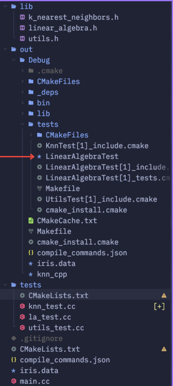
Project Overview
your-cool-project-name/
├── CMakeLists.txt
├── lib
│ ├── k_nearest_neighbors.h
│ ├── linear_algebra.h
│ └── utils.h
├── tests
│ ├── CMakeLists.txt
│ ├── knn_test.cc
│ ├── la_test.cc
│ └── utils_test.cc
├── main.cc
└── iris.data
In this project, we have a lib folder containing our core functionalities. The tests folder includes testing files for each individual file created in the lib directory.
Make sure to download the Iris dataset for your project.
Setting up CMake
For our project, we've chosen CMake as our build system generator. If you're not familiar with CMake, you can find a helpful introduction here.
To streamline the CMake process, I use cmake_tool_nvim to assist in generating and building our project. If you're using VSCode or CLion, there are plugins and built-in features available to support CMake integration.
Remember to run the CMake Generate command before you start coding. Similar to using a package manager, this step is crucial for including dependencies. Once generated, you can choose which executable to build or run directly.
Here's the CMake configuration for ./CMakeLists.txt (not in test folder):
cmake_minimum_required(VERSION 3.5)
project(knn_cpp CXX)

# Set up C++ version and properties
include(CheckIncludeFileCXX)

check_include_file_cxx(any HAS_ANY)
check_include_file_cxx(string_view HAS_STRING_VIEW)
check_include_file_cxx(coroutine HAS_COROUTINE)

set(CMAKE_CXX_STANDARD 20)
set(CMAKE_BUILD_TYPE Debug)
set(CMAKE_CXX_STANDARD_REQUIRED ON)
set(CMAKE_CXX_EXTENSIONS OFF)

# Copy data file to build directory
file(COPY ${CMAKE_CURRENT_SOURCE_DIR}/iris.data DESTINATION ${CMAKE_CURRENT_BINARY_DIR})

# Download library usinng FetchContent
include(FetchContent)

FetchContent_Declare(matplotplusplus
        GIT_REPOSITORY https://github.com/alandefreitas/matplotplusplus
        GIT_TAG origin/master)

FetchContent_GetProperties(matplotplusplus)
if(NOT matplotplusplus_POPULATED)
  FetchContent_Populate(matplotplusplus)
  add_subdirectory(${matplotplusplus_SOURCE_DIR} ${matplotplusplus_BINARY_DIR} EXCLUDE_FROM_ALL)
endif()

FetchContent_Declare(
    fmt
    GIT_REPOSITORY https://github.com/fmtlib/fmt.git
    GIT_TAG        7.1.3  # Adjust the version as needed
)

FetchContent_MakeAvailable(fmt)

# Add executable and link project libraries and folders
add_executable(${PROJECT_NAME} main.cc)

target_link_libraries(${PROJECT_NAME} PUBLIC matplot fmt::fmt)

aux_source_directory(lib LIB_SRC)

target_include_directories(${PROJECT_NAME} PRIVATE ${CMAKE_CURRENT_SOURCE_DIR})

target_sources(${PROJECT_NAME} PRIVATE ${LIB_SRC})

add_subdirectory(tests)
In our cmake we need 3 parts:
- Set up C++ version and properties
- Use FetchContent to download libraries
- Add executable and link project libraryies and folders
As modern CMake we don't actually need to clone library and build it into your local. We can use FetchContent to download the library we need for our projects.
Here's the CMake configuration for ./tests/CMakeLists.txt:
cmake_minimum_required(VERSION 3.5)
project(knn_cpp CXX)

include(FetchContent)
FetchContent_Declare(
  googletest
  GIT_REPOSITORY https://github.com/google/googletest.git
  GIT_TAG release-1.11.0
)
FetchContent_MakeAvailable(googletest)

FetchContent_Declare(matplotplusplus
        GIT_REPOSITORY https://github.com/alandefreitas/matplotplusplus
        GIT_TAG origin/master)

FetchContent_GetProperties(matplotplusplus)
if(NOT matplotplusplus_POPULATED)
  FetchContent_Populate(matplotplusplus)
  add_subdirectory(${matplotplusplus_SOURCE_DIR} ${matplotplusplus_BINARY_DIR} EXCLUDE_FROM_ALL)
endif()

function(knn_cpp_test TEST_NAME TEST_SOURCE)
  add_executable(${TEST_NAME} ${TEST_SOURCE})

  target_link_libraries(${TEST_NAME} PUBLIC matplot)

  aux_source_directory(${CMAKE_CURRENT_SOURCE_DIR}/../lib LIB_SOURCES)

  target_link_libraries(${TEST_NAME} PRIVATE gtest gtest_main gmock gmock_main)

  target_include_directories(${TEST_NAME} PRIVATE ${CMAKE_CURRENT_SOURCE_DIR} ${CMAKE_CURRENT_SOURCE_DIR}/../)

  target_sources(${TEST_NAME} PRIVATE ${LIB_SOURCES} )

  include(GoogleTest)
  gtest_discover_tests(${TEST_NAME})

endfunction()

knn_cpp_test(LinearAlgebraTest la_test.cc)
knn_cpp_test(KnnTest knn_test.cc)
knn_cpp_test(UtilsTest utils_test.cc)
Now, let's continue with our project without getting too deep into the details of CMake setup. (Just copy it 😑)
Create Knn model
To create a Knn model, we follow these three steps:
Utils functions:
We need utility functions to split the dataset and a TupleHash to support using a Tuple as a key in a HashMap.Distance calculation:
Implement a function to calculate the distance between an evaluated point and a training point. This is a crucial step in our Knn algorithm.Knn model:
Develop the Knn model itself, which involves calculating the most voted class based on the nearest neighbors.
These steps are the building blocks of our Knn model and will be the core of our implementation. Let's do each step one at a time.
Utils functions
Let's move to ./utils.h. The reason I only use header because you know I'm lazy let's put everything inside header for import purpose. This style I copy from PezzzasWork when I try to copy his Ant simulation code hehehe 😅.
// utils.h
#include <algorithm>
#include <cstddef>
#include <random>
#include <vector>

template <typename T>
std::pair<std::vector<T>, std::vector<T>> split_data(const std::vector<T> &data,
                                                     double prob) {
  std::random_device rd;
  std::mt19937 g(rd());

  std::vector<T> shuffled_data = data;
  std::shuffle(shuffled_data.begin(), shuffled_data.end(), g);

  auto cut = static_cast<size_t>(data.size() * prob);

  std::vector<T> train(shuffled_data.begin(), shuffled_data.begin() + cut);
  std::vector<T> test(shuffled_data.begin() + cut, shuffled_data.end());

  return std::make_pair(train, test);
}

struct TupleHash {
  template <class T1, class T2>
  std::size_t operator()(const std::tuple<T1, T2> &p) const {
    auto hash1 = std::hash<T1>{}(std::get<0>(p));
    auto hash2 = std::hash<T2>{}(std::get<1>(p));
    return hash1 ^ hash2;
  }
};
As mentioned earlier, we need two functions. The first one is split_data(data, prob). This function divides our data into training and testing sets based on the provided probability parameter. To kick things off, we start by shuffling our data. Next, we find the cut-off position by multiplying the length of the dataset by the probability. Finally, we split the data into training and testing vectors using the begin() and end() iterators.
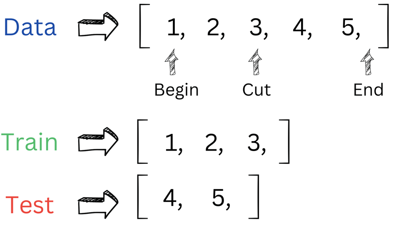
Here's an example to illustrate how the 'cut' works. It's quite similar to dealing with a nested vector; we're just need to replace vector vector<int> with vector<vector>.
And for reference, here's how our Python does it:
# This is python code from https://github.com/joelgrus/data-science-from-scratch/blob/master/scratch/machine_learning.py

def split_data(data: List[X], prob: float) -> Tuple[List[X], List[X]]:
    """Split data into fractions [prob, 1 - prob]"""
    data = data[:]                    # Make a shallow copy
    random.shuffle(data)              # because shuffle modifies the list.
    cut = int(len(data) * prob)       # Use prob to find a cutoff
    return data[:cut], data[cut:]     # and split the shuffled list there.
The second one is not exactly a function but a defined struct. Yeah, I might have lied a bit there 😜. This struct allows us to use a tuple as a hash key, which will come in handy when we come into visualization. For now, let's just leave it be.
Linear Algebra (Distance between two vector)
Let's move to ./linear_algebra.h.
A major part of Knn is that we need something to define a features or vectors of data is part of specific neighbors. The usual way is to calculating the distance from the evaluated vector to every vector in the dataset. This process helps us identify the closest neighbors based on distance.
d(X, Y) = sqrt((x₁ - y₁)² + (x₂ - y₂)² + ... + (xn - yn)²)
You can find this formula here
Here, X and Y (X -> vector X and Y -> vector Y) represent features of our data , such as Sepal length, Sepal width, etc.
// linear_algebra.h
#include <cassert>
#include <vector>

typedef std::vector<double> Vector;

namespace linear_algebra {

inline Vector subtract(const Vector &v, const Vector &w) {
  assert(v.size() == w.size() && "vectors must be the same length");
  Vector result(v.size());
  for (size_t i = 0; i < v.size(); ++i) {
    result[i] = v[i] - w[i];
  }
  return result;
}

inline double dot(const Vector &v, const Vector &w) {
  assert(v.size() == w.size() && "vectors must be the same length");
  double result = 0.0;
  for (size_t i = 0; i < v.size(); ++i) {
    result += v[i] * w[i];
  }
  return result;
}

inline double sum_of_squares(const Vector &v) { return dot(v, v); }

inline double magnitude(const Vector &v) { return sqrt(sum_of_squares(v)); }

inline double distance(const Vector &v, const Vector &w) {
  return magnitude(subtract(v, w));
}

} // namespace linear_algebra
To keep things organized, we'll break down the distance calculation into smaller functions:
-
subtract: subtract corresponding elements of two vectors. -
dot: calculate the dot product of two vectors. -
sum_of_squares: compute the sum of squares of vector elements. -
magnitude: find the magnitude of a vector
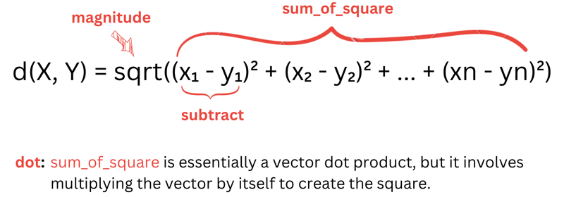
While we could combine everything into the distance function, organizing these smaller functions separately makes our code cleaner and more reuseable. These functions will come in handy, and who knows, distance might be the only one to use them.
Knn (K-nearest neighbors algorithm)
Let's move to ./k_nearest_neighbors.h.
Now that we've wrapped up the basics with utils and linear algebra, it's time to dive into the K-nearest neighbors (Knn) algorithm. Those earlier sections were just a easy part! 😅 But don't worry; as we break down each small part, things will start to become clearer. Understanding something might take some time—It took me few days to understand it (Don't expect to understand something in one day that takes years for someone to discover). So, take your time, there's no rush, and no one is going to force you anyway 😆.
// k_nearest_neighbors.h
#include "linear_algebra.h"
#include <algorithm>
#include <cstdlib>
#include <string>
#include <unordered_map>
#include <vector>

struct LabelPoint {
  Vector point;
  std::string label;
};

namespace knn {

template <typename T> T majority_vote(const std::vector<T> &labels) {
  std::unordered_map<T, size_t> vote_counts;
  for (const T &label : labels) {
    vote_counts[label]++;
  }

  auto max_vote = std::max_element(
      vote_counts.begin(), vote_counts.end(),
      [](const auto &a, const auto &b) { return a.second < b.second; });

  size_t winner_count = max_vote->second;
  size_t num_winners = std::count_if(vote_counts.begin(), vote_counts.end(),
                                     [winner_count](const auto &entry) {
                                       return entry.second == winner_count;
                                     });

  if (num_winners == 1) {
    return max_vote->first;
  } else {
    return majority_vote(std::vector<T>(labels.begin(), labels.end() - 1));
  }
}

inline std::string knn_classify(int k,
                                const std::vector<LabelPoint> &labeled_points,
                                const Vector &new_point) {
  auto by_distance = labeled_points;
  std::sort(by_distance.begin(), by_distance.end(),
            [new_point](const auto &lp1, const auto &lp2) {
              return linear_algebra::distance(lp1.point, new_point) <
                     linear_algebra::distance(lp2.point, new_point);
            });

  std::vector<std::string> k_nearest_labels;
  k_nearest_labels.reserve(k);
  for (int i = 0; i < k; ++i) {
    k_nearest_labels.push_back(by_distance[i].label);
  }

  return majority_vote(k_nearest_labels);
}

} // namespace knn
Now this look overwhelming. Let's visualize and break down every small part of it.
LabelPoint Class:
First one is LabelPoint. This class lets us store the features and labels of each row in our dataset in a simple struct.
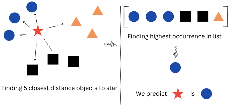
majority_vote Function:
Moving on to the second part - the majority_vote function. As mentioned earlier, in Knn, we calculate the most voted class based on the nearest neighbors. This function helps us find the most frequent value in the entire training dataset, essentially the one that appears the most in the array.
-
vote_countsis a hash map storing the occurrences of each value (because, well, who doesn't solve problems with a hash map? 😏). - We use
std::max_elementto find the highest occurrence in our map. The result,max_vote, contains the key (max_vote.first) and the value (max_vote.second) of the most frequent element. - The value (
max_vote.second) is stored inwinner_count. - Next, we count how many elements in our map have the same value as
winner_countusingstd::count_if. - If there's only one element, we return its key (label).
- If not, we eliminate one element at a time and repeat the process until we find a unique winner.
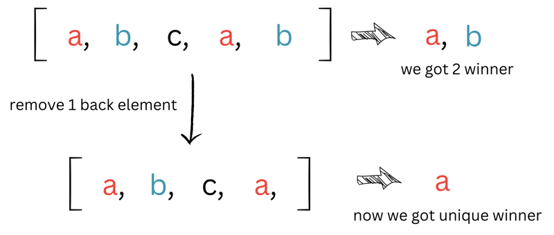
There are several ways to choose a unique winner, some suggested by Joel Grus in his book:
- Pick one of the winners at random.
- Weight the votes by distance and pick the weigthed winner.
- Reduce
kuntil we find a unique winner (this is the one we chose).
But you may wonder if k is too big, our code will be too slow. However, the way we choose k is relatively small because we only choose the top 5, 10, or 20 at most. So this is not a big problem for us.
knn_classify Function:
Now, let's discuss the knn_classify function, a key player in our prediction process. This function scans every point in the training dataset and selects the top k points that are closest to the new_point.
Here's what happens step by step:
We sort our points based on their distance to the new_point.
We then pick the top k points that are closest to the new_point.
Finally, we determine the label of the point that appears most frequently in the selected array.
This part of the code might be a bit confusing:
  std::sort(by_distance.begin(), by_distance.end(),
            [new_point](const auto &lp1, const auto &lp2) {
              return linear_algebra::distance(lp1.point, new_point) <
                     linear_algebra::distance(lp2.point, new_point);
            });
Here, we're using std::sort, but we're doing a custom comparison using the distance function. It sorts the points based on how close they are to the new_point, so the point with the closest distance ends up at the beginning of the array. You can read about this sort here
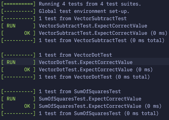
Testing our code
After completing various tasks, it's time to test our code to ensure everything works as intended.
Navigate to the ./tests/ folder to find the testing code. The tests mainly consist of simple if-else statements. Feel free to explore these code snippets yourself.
// ./test/utils_test.c
#include <gmock/gmock.h>
#include <gtest/gtest.h>
#include <lib/utils.h>
#include <numeric>
#include <vector>

TEST(SplitDataTest, ExpectedCorrectValue) {
  std::vector<int> data(1000);
  std::iota(data.begin(), data.end(), 0);

  auto [train, test] = split_data(data, 0.75);

  EXPECT_EQ(train.size(), 750);
  EXPECT_EQ(test.size(), 250);

  std::vector<int> combined_data(train.begin(), train.end());
  combined_data.insert(combined_data.end(), test.begin(), test.end());
  std::sort(combined_data.begin(), combined_data.end());

  for (size_t i = 0; i < combined_data.size(); ++i) {
    EXPECT_EQ(combined_data[i], static_cast<int>(i));
  }
}
// ./test/la_test.cc
#include <gtest/gtest.h>
#include <lib/linear_algebra.h>

TEST(VectorSubtractTest, ExpectCorrectValue) {
  Vector v{5, 7, 9};
  Vector w{4, 5, 6};

  Vector result = linear_algebra::subtract(v, w);

  EXPECT_EQ(result, Vector({1, 2, 3}));
}

TEST(VectorDotTest, ExpectCorrectValue) {
  Vector v{1, 2, 3};
  Vector w{4, 5, 6};

  double result = linear_algebra::dot(v, w);

  EXPECT_EQ(result, 32);
}

TEST(SumOfSquaresTest, ExpectCorrectValue) {
  Vector v{1, 2, 3};

  double result = linear_algebra::sum_of_squares(v);

  EXPECT_EQ(result, 14);
}

TEST(MagnitudeTest, ExpectCorrectValue) {
  Vector v{3, 4};

  double result = linear_algebra::magnitude(v);

  EXPECT_EQ(result, 5);
}
// ./test/knn_test.cc
#include <gmock/gmock.h>
#include <gtest/gtest.h>
#include <lib/k_nearest_neighbors.h>
#include <string>
#include <vector>

TEST(MajorityVote, ExpectedCorrectValue) {
  std::vector<std::string> labels_majority = {"a", "b", "c", "a", "b"};
  EXPECT_EQ(knn::majority_vote(labels_majority), "a");
}
If you want to run these remember to select build target arcoding to name we gave them in our ./tests/CMakeLists.txt
...Rest of above code

knn_cpp_test(LinearAlgebraTest la_test.cc)
knn_cpp_test(KnnTest knn_test.cc)
knn_cpp_test(UtilsTest utils_test.cc)
Building and Running:
Once you've finished writting tests, it's time to run your CMake build in your editor to generate the specific executable. In my case, I use :CMakeSelectBuildTarget followed by :CMakeBuild. After this process, the executable file will be created in your debug folder.
Testing Execution:
To test our code, navigate to the Debug folder using the cd command and run ./LinearAlgebraTest. You can follow the same process for the rest of your tests.
Here is the result:
Putting everything together
Let's move to ./main.cc
Since the ./main.cc file is quite lengthy, I'll show each part one at a time.
parse_iris_row
// ./main.cc
#include <iostream>
#include <lib/k_nearest_neighbors.h>
#include <lib/utils.h>
#include <fmt/core.h>
#include <matplot/matplot.h>

LabelPoint parse_iris_row(const std::vector<std::string> &row) {
  std::vector<double> measurements;
  for (size_t i = 0; i < row.size() - 1; ++i) {
    measurements.push_back(std::stod(row[i]));
  }

  std::string label = row.back().substr(row.back().find_last_of("-") + 1);

  return LabelPoint{measurements, label};
}
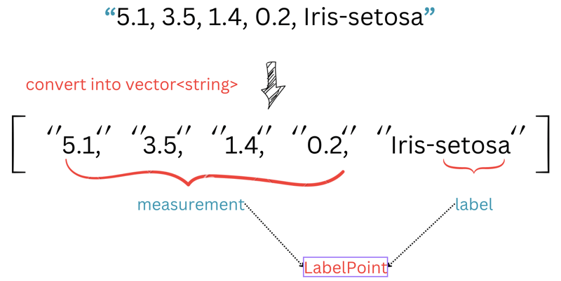
If you look at each row in our ./iris.data, you will see each row has 5 elements. The first 4 elements represent iris sepal and petal measurements, and the last one is the iris type.
In this code, we extract the first 4 elements as std::vector<double> for measurements, and the last element is extracted for label. We then return these values as a LabelPoint. You may ask "what is this weird code here?".
std::string label = row.back().substr(row.back().find_last_of("-") + 1);
This code helps us retrieve only the name of the iris. For example, if the original name is Iris-virginica, we only need virginica without the Iris prefix.
Now let's code our knn pipeline!.
Knn pipeline
This function happens to be the longest in our entire code. Well, blame it on my laziness, but I decided to throw everything in here 😏.
Alright, let's break down our code. In this function, we have four sections:
-
Extracting Data from
iris.data:- We use
std::ifstreamto read data from theiris.datafile.
- We use
-
Plotting and Visualizing Data:
- We use
matplotplusplusto create plots and visualize our data.
- We use
-
Splitting and Predicting using
knn_classify:- We use the
split_datafunction to split andknn_classifyto predict.
- We use the
-
Plotting our Confusion Matrix:
- Finally, we create a plot for our confusion matrix.
Extracting Data
Let's extract our data from iris.data and store it in a vector of LabelPoint for later use. The following code demonstrates how to achieve this:
// ./main.cc
void testing_knn() {
  // Extract data
  std::ifstream file("./iris.data");
  std::string line;

  std::vector<LabelPoint> iris_data;

  if (file.is_open()) {
    while (std::getline(file, line)) {
      std::istringstream iss(line);
      std::vector<std::string> row;

      while (iss) {
        std::string value;
        if (!std::getline(iss, value, ',')) {
          break;
        }
        row.push_back(value);
      }

      if (!row.empty()) {
        iris_data.push_back(parse_iris_row(row));
      }
    }

    file.close();
  } else {
    std::cerr << "Unable to open file\n";
  }
}
The first while loop is a basic stream reading operation in C++. You can find it here. The second while loop separates each element using the specified delimiter. You can also find it here. After that, we store everything in row, which is a vector<string>. Lastly we parse this row into LabelPoint
Plotting and Visualizing Data
Now come to the most pain in the ass, plotting using matplotplusplus, it take me quite a few attempts to get it right! 🥲. But I'll only show you the one that worked - hiding my own failure 😆.
// ./main.cc

void test_knn() {
// Rest of above code

  std::map<std::string, std::vector<Vector>> points_by_species;
  for (const auto &iris : iris_data) {
    points_by_species[iris.label].push_back(iris.point);
  }

  std::vector<std::string> metrics = {"sepal length", "sepal width",
                                      "petal length", "petal width"};
  std::vector<std::pair<int, int>> pairs;
  std::vector<std::string> marks = {"+", ".", "x"};

  for (int i = 0; i < 4; ++i) {
    for (int j = i + 1; j < 4; ++j) {
      pairs.push_back(std::make_pair(i, j));
    }
  }

  matplot::tiledlayout(2, 3);
  for (size_t p = 0; p < pairs.size(); ++p) {
    int i = pairs[p].first;
    int j = pairs[p].second;
    auto sp = matplot::nexttile();
    sp->title(fmt::format("{} vs {}", metrics[i], metrics[j]));
    for (size_t m = 0; m < marks.size(); ++m) {
      const auto &[species, points] = *std::next(points_by_species.begin(), m);
      Vector xs, ys;
      for (const auto &point : points) {
        xs.push_back(point[i]);
        ys.push_back(point[j]);
      }
      matplot::scatter(xs, ys)->marker(marks[m]).display_name(species);
      matplot::hold(true);
    }
  }
  matplot::legend("lower right")
      ->location(matplot::legend::general_alignment::bottomright);
  matplot::legend()->font_size(6);
  matplot::show();
}
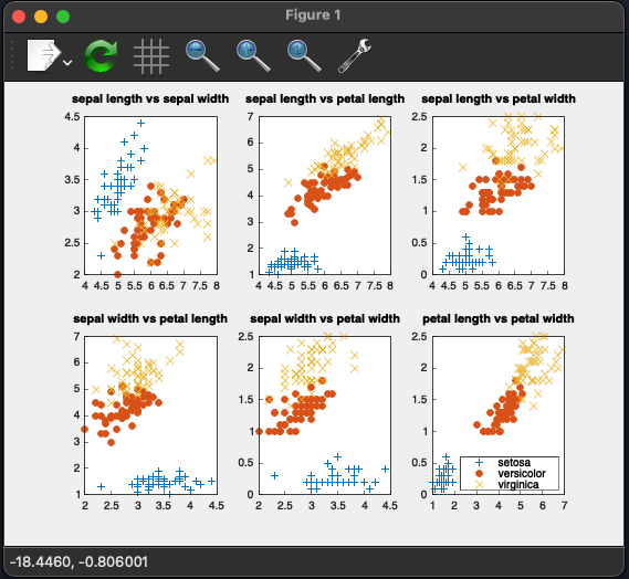
The first task in data science is often plotting our data. In this code, we use matplotplusplus as an alternative to Matplotlib in Python.
The first thing you'll encounter is points_by_species, which stores labels as keys and points as list of vectors of measurements. After this, points_by_species will have 3 keys (because we have 3 species to handle).
Next, we create 6 pairs of measurements. This is similar to finding subsets of an array. Each pair looks like this: [{0, 1}, {0, 2}, {0, 3}, {1, 2}, ...]. We set 0 as sepal length, 1 as sepal width, 2 as petal length, and 3 as petal width.
Then, we proceed to plot each pair of measurements.
for (size_t m = 0; m < marks.size(); ++m) {
      const auto &[species, points] = *std::next(points_by_species.begin(), m);
      // Rest of below code
}
In this loop, I use std::next to iterate through every key in the map. Remember that points is a list of vectors of measurements, and point is a vector of measurements that contains exactly 4 elements: sepal length, sepal width, petal length, and petal width.
If you choose the CMake build target as knn_cpp, build and run it, you will see the following result:
Splitting and Predicting
Before we proceed with the next code, let's comment out the entire Plotting and Visualizing Data section. This will prevent overlapping plots, and unfortunately, I have no idea how to fix it 😢. (You can follow the same way as I did in my repository).
Now, let's dive into predicting Iris types using our created knn model.
// ./main.cc
void test_knn(){

// Rest of above code

  std::srand(12);

  auto split_result = split_data(iris_data, 0.70);

  const std::vector<LabelPoint> &iris_train = split_result.first;
  const std::vector<LabelPoint> &iris_test = split_result.second;

  assert(iris_train.size() == static_cast<size_t>(0.7 * iris_data.size()));
  assert(iris_test.size() == static_cast<size_t>(0.3 * iris_data.size()));

  std::unordered_map<std::tuple<std::string, std::string>, int, TupleHash>
      confusion_matrix;
  int num_correct = 0;

  for (const auto &iris : iris_test) {
    std::string predicted = knn::knn_classify(5, iris_train, iris.point);
    std::string actual = iris.label;

    if (predicted == actual) {
      num_correct++;
    }

    confusion_matrix[{predicted, actual}]++;
  }

}
In this code block, we split our data using split_data into a 70% training set and a 30% test set.
Next, we create a for loop to predict every test data in our test set. We also store our predictions in the confusion matrix and increase num_correct if it's correct. You can read about the confusion matrix here.
Plotting our Confusion Matrix
Now let's plot our confusion matrix
// ./main.cc
void test_knn() {

// Rest of above code

  double pct_correct = static_cast<double>(num_correct) / iris_test.size();
  std::cout << pct_correct << std::endl;

  std::vector<std::string> labels = {"setosa", "versicolor", "virginica"};
  std::vector<std::vector<double>> counts(
      labels.size(), std::vector<double>(labels.size(), 0));

  for (const auto &entry : confusion_matrix) {
    const auto &key = entry.first;
    size_t predicted_index =
        std::find(labels.begin(), labels.end(), std::get<0>(key)) -
        labels.begin();
    size_t actual_index =
        std::find(labels.begin(), labels.end(), std::get<1>(key)) -
        labels.begin();
    counts[predicted_index][actual_index] = static_cast<double>(entry.second);
  }

  matplot::gca()->children({});

  matplot::heatmap(counts);
  matplot::title("Confusion Matrix Heatmap");
  auto ax = matplot::gca();
  ax->x_axis().ticklabels(labels);
  ax->y_axis().ticklabels(labels);
  matplot::xlabel(ax, "Actual Labels");
  matplot::ylabel(ax, "Predicted Labels");
  matplot::show()
}
This code block helps us plot our confusion matrix and show the accuracy of our model.
The most important part is this section:
 std::vector<std::string> labels = {"setosa", "versicolor", "virginica"};
  std::vector<std::vector<double>> counts(
      labels.size(), std::vector<double>(labels.size(), 0));

  for (const auto &entry : confusion_matrix) {
    const auto &key = entry.first;
    size_t predicted_index =
        std::find(labels.begin(), labels.end(), std::get<0>(key)) -
        labels.begin();
    size_t actual_index =
        std::find(labels.begin(), labels.end(), std::get<1>(key)) -
        labels.begin();
    counts[predicted_index][actual_index] = static_cast<double>(entry.second);
  }
where we need to map our confusion matrix to some like this
std::vector<std::vector<double>> data = {
        {45, 60, 32}, {43, 54, 76}, {32, 94, 68}, {23, 95, 58}};
You can read more about it here
As you see we need to create labels as vector of string, we need to this one for converting our label string into index number, and below for loop is to convert our std::unordered_map<std::tuple<std::string, std::string>, int, TupleHash> confussion_matrix into std::vector<std::vector<double>> counts.
Here, we create labels as a vector of strings, and we use this to convert our label strings into index numbers. The subsequent for loop is responsible for converting our std::unordered_map<std::tuple<std::string, std::string>, int, TupleHash> confusion_matrix into std::vector<std::vector<double>> counts.
Again if you choose the CMake build target as knn_cpp, build and run it, you will see the following result with accuracy above 90%:
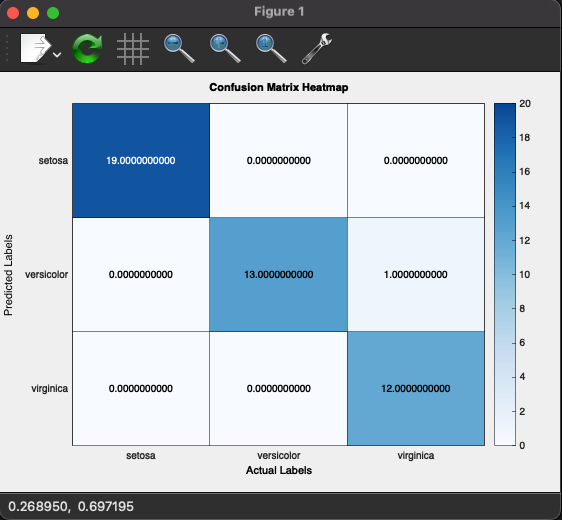
You may notice errors, mostly with versicolor and virginica types. These two are very similar, as highlighted in the visualizing our data section where they sometimes overlap. The main difference is their color, but unfortunately, our dataset doesn't include such a field.
Conclusion
We successfully built our knn model from scratch using only C++. I know that my explanations might be lacking, especially in the last section. making me question if I truly understand them. Your feedback is invaluable, and I welcome any suggestions to improve. While this project may seem silly, I found it challenging to implement in C++ from scratch. Despite not achieving anything, I'm still happy with it.
I appreciate your patience in reaching this section. I know that my writing skills is very bad. If you encounter any difficulties, please feel free to comment below, and I'll gladly help you.
Thank you for your time and understanding.

Top comments (0)