In this final blog post, I will get quite specific, as I try to convey the specifics of my thesis project, "Privacy-preserving Similarity Search", in which I designed and analyzed an algorithm - more specifically a differentially private one. You are not meant to understand everything in this blog post. It serves an inspirational purpose through a real world example of the process of designing an algorithm. However, if you have time for it, I encourage you to pause, anytime you read something, which you are not familiar with, and learn that concept or term before continuing.
Let’s start out with an introduction to a new class of algorithms, namely randomized algorithms, which our algorithm falls under.
Randomized Algorithms
Randomized algorithms are based on a bunch of probabilistic theories, which we will not get into. True randomness is also left for another discussion. My goal is simply to demonstrate the capabilities and advantages of introducing randomness in the design of an algorithm, allowing for random decisions when processing a given input. As opposed to the deterministic algorithms we have seen so far, neither the same output nor running time can be guaranteed for the same input to a randomized algorithm.
So why do we strengthen the underlying model of our algorithm, when we introduce randomness? It differs from algorithm to algorithm. Oftentimes the strength lies in a conceptually simpler algorithm, where less internal state or memory is required, or in an alleviation of certain worst-case scenarios. Let us look at an example of the latter.
For the sake of the example, we will look into the quicksort algorithm, as the approach of the algorithm is easily conceptualized.
The algorithm is a divide and conquer algorithm, in which a pivot in a list is initially chosen - typically the first, middle, or last element. Then it divides the remaining elements into two sublists based on whether the elements are smaller (illustrated by the green array) or larger (illustrated by the blue array) than the pivot. Then The same process is then repeated for each sub array (recursively), until the entire array is sorted. This is visualized both during and after sorting for two different elements of two different lists.

In quicksort, randomization is simply introduced by choosing the pivot at random. Why is this an advantage? First, I encourage you to prove that the optimal scenario for the quicksort algorithm is one, where the algorithm repeatedly divides the array into two equal-sized subarrays.
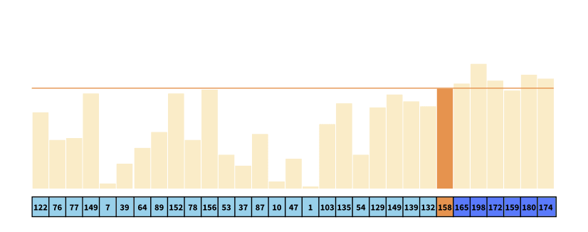
Now, Imagine the following worst-case scenario. Consider an implementation of the algorithm, in which the first element is always chosen as the pivot, as well as an array which is sorted in decreasing order as depicted in the visualization. Given an array of size n (here n = 30), the algorithm partitions the array into one subarray of size n-1, which is the exact opposite of the optimal partition of the array.

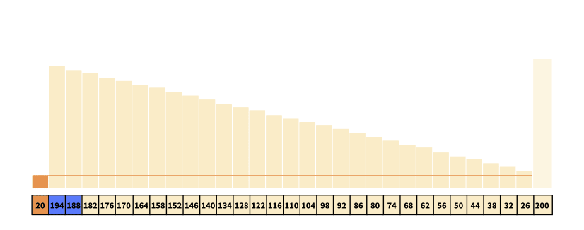
Introducing randomness in picking the pivot, we could alleviate certain worst-case scenarios like these, which actually improves the expected or average time complexity. However, even though we improve the average-time complexity, we still cannot improve the worst-case complexity, which is still O(n2), as the random pivot could still repeatedly be chosen as the first element in the example above.
I strongly encourage you to watch the following series of animations, to visualize the algorithm as well as the randomization hereof: https://www.chrislaux.com/quicksort.html.

Differential Privacy
The goal of differential privacy is to permit statistical analysis of a database or population, without compromising the privacy of the individuals who partake. More specifically, it strives towards ensuring that the same conclusion is reached independently of the presence or absence of any individual in said population. Hereby, an individual can partake in a statistical analysis without incurring any risk of compromising the privacy of said individual.
So why did we introduce randomized algorithms? Differential privacy is not an algorithm, but a definition of privacy tailored for private data release. The algorithms, which fall under this definition, utilizes randomized algorithms, as it will provide privacy by introducing randomness.
Differential privacy exists in both a localized and a centralized manner. We will only look into centralized differential privacy, in which a centralized trusted curator ensures the privacy of the individuals by applying a differentially private algorithm to the conclusions of any statistical query on the population.
Let us look at an example of a very simple differentially private randomized algorithm to conceptualize these guarantees, and to see how randomization can help us in complying with these guarantees.
In the algorithm randomized response, participants are asked whether or not they have some property p (e.g. diabetes). They are then asked to answer using the following approach,
- Flip a coin.
- If tails, then respond truthfully.
- If heads, then flip a second coin and respond “yes”, if heads, or “no”, if tails.
As Dwork and Roth ([16], p. 30) states, the privacy of this algorithm originates from the randomness and the plausible deniability of any response, as an answer of “yes”, can be either truthful, or the result of two flips of heads, with a probability of ¼, independently of whether the participant has property p or not. Try to convince yourself, that this, as well as the opposite case (i.e. "no"), is true.
It becomes increasingly harder to guarantee the same level of privacy, as the number of participants decrease, seeing as the dependency of each individual on the conclusion of a statistical analysis inherently increases. Intuitively, and in a simplified manner, one would then imagine that the smaller the population is, the more noise should be added to any statistical query over said population, to ensure the same level of privacy.
To determine the amount of noise needed to maintain the same level of privacy, we introduce an important parameter in differential privacy. The parameter epsilon, ε, captures the probability of reaching the same conclusion, where a smaller ε would yield better privacy, but less accurate conclusions. This parameter is called privacy loss and is interesting, as it makes privacy a quantifiable measure.
An algorithm is said to be ε-differentially private, if for any pair of datasets that differ by a single element or individual, the probability of reaching the same conclusion on the two datasets differs by no more than eε.
Let us end our introduction of differential privacy by looking at some of its many qualitative properties.
First and most importantly, it enables a quantification of privacy, by the privacy loss parameter, ε, which is notable, as privacy is often considered as a binary concept.
Second, it neutralizes any linkage attacks based on past, present, or even future data. In a linkage attack, one tries to de-anonymize individuals by comparing different datasets, most recently known from the Netflix Prize, https://en.wikipedia.org/wiki/Netflix_Prize.
Third and lastly, it enables composition of the previously mentioned privacy loss. This means that we are able to extend our quantification of privacy to the privacy loss of multiple queries in a cumulative manner.
Given this very brief introduction to randomized algorithms and differential privacy, we will dive right into the design and analysis of the differentially private algorithm, which I developed in my thesis project.
Privacy-preserving Similarity Search
We have now finally reached our real world example of the design and, to some extent analysis, of an algorithm. Let's get into our differentially private algorithm. This chapter is very technical and uses theory, which is not previously introduced. I hope it will still give you a valuable perspective on what is possible in the world of algorithms.
In my thesis project, entitled "Privacy-preserving Similarity Search", my thesis partner and I proposed and implemented a private data release mechanism (an algorithm), for applying differential privacy in a similarity search setting. We then evaluated the quality of the mechanism for nearest neighbor search on private datasets by comparing it with another mechanism developed by Dhaliwal et al. (https://arxiv.org/pdf/1901.09858.pdf).
An understanding of similarity search, and nearest neighbor search in particular, is not necessary, as it merely served as an exemplary domain for our mechanism.
We will only go into the details with the design of the algorithm, as the complexity of the analysis exceeds the purpose of this blogpost. However, in our report, which I will gladly email to anyone interested, we do prove that our algorithm is (ε, δ)-differentially private, that the mechanism is an unbiased estimator maintaining distances in expectation, and present guarantees for the precision of the estimation by means of Chebyshev bounds.
Design considerations
Let’s get into the design and implementation of the algorithm. Differential privacy algorithms usually consist of two stages - first the original data is transformed by reducing the dimensionality, then, a certain amount of noise is added to make the data private. In a centralized setting, where a trusted curator handles queries on the population, the steps can be depicted as seen in the visualization.

Before introducing the algorithm, I will introduce one final piece of theory, which we use in the first stage of our algorithm.
We want to reduce the dimensionality of our data. Let’s imagine that our data consists of a matrix, where each row represents a participant and each column represents some answer or characteristic of said participant.
To transform said data, we adapted the SimHash algorithm (https://www.cs.princeton.edu/courses/archive/spr04/cos598B/bib/CharikarEstim.pdf). Our main reason for choosing this algorithm is its ability to preserve distances (in terms of similarity search domain) despite projecting the data into a binary format, which makes it less spatially expensive.
The algorithm falls under the Locality Sensitive Hashing framework, which is based on the principle that if two data points are close, based on some similarity function, then their respective hash values are also close. This means, as opposed to conventional hashing, that collisions for similar items are maximized, which is certainly favorable in a similarity search setting.
The algorithm is based upon a collection of random d-dimensional vectors, r in Rd, where each coordinate is drawn from a Gaussian distribution. Given a random vector, r, and some vector, u, of the original dataset, the hash functions of the algorithm is defined as follows,

Therefore, using the dot product between the random vector, r, and the vector, u, from the original dataset, it is encoded whether u falls on one side (1) or the other (0) of the random vector, r. By increasing the number of hash functions we apply to the vector, we can decrease the probability of collision of hash values of dissimilar vectors. Again, this got really technical, but try to convince yourself of this using the illustration below, where we have applied two hash functions, based on two random vectors, r1 and r2, to three different vectors of the original dataset for comparison.

Designing the algorithm
It is finally time to introduce the algorithm. I will start by formally introducing our SimRand algorithm, thereafter I will explain the algorithm, step by step.

First, let's go through the input and output of the algorithm. The input of the algorithm consists of an original dataset X, a matrix with n rows and d columns, a target dimensionality k for our dimensionality reduction, epsilon and delta values representing the privacy loss, and finally a alpha value representing an upper bound on the angle between two neighboring vectors (or databases) - neighboring databases will be defined in terms of the sensitivity of a query shortly). The output of the algorithm is a differentially private dataset Z.
Let’s go through the algorithm step by step. We will use an example dataset consisting of a single vector to explain the steps of the algorithm.

In the first step, we create projection matrix, R, which is effectively used to reduce the dimensionality (i.e. the number of columns) of our original dataset from d to k, in our case from 8 to 6 columns.

In the second step, we reduce the dimensionality of our original dataset, creating a new matrix, Y, by matrix multiplication between the projection matrix, R, and the original matrix, X, which in our case is simplified to a vector (i.e. one row). Effectively, each coordinate of Y represents the dot product between the vector of X and the columns of R. Our new reduced matrix Y is now a vector of 6 columns.

In the third step, we effectively transform the matrix, Y, into a binary matrix, ^Y, based on the sign of the dot product between each coordinate of the matrices X and R in Y. Each coordinate is represented by a 1 if the angle between the vectors is less than 90 degrees.

We have now reduced the dimensionality of the original dataset and projected it into a binary format. Now, we need to add noise to make the data private. But how much noise should we add? As discussed early in our introduction, more noise means more privacy, but also lower accuracy.
It turns out that the amount of noise added, depends on the sensitivity of the function or query, which we want to apply to our dataset. The sensitivity of a function represents the largest possible difference that one row can have on the result of that function or query, for any dataset, which by definition of differential privacy is exactly what we are trying to conceal. The sensitivity of a query, which simply counts the number of rows, or participants, in a dataset has a sensitivity of 1, as adding or removing a single row from any dataset will change the count by at most 1. It turns out, that the sensitivity also defines neighboring database - in our example if two databases differ in no more than one row.
In our fourth step, we calculate the sensitivity K, i.e. the maximum number of places, where two vectors differ, which intuitively can be no larger than the dimensionality of the two vectors.

In our fifth step, using K, we can now calculate the probability p that two coordinates collide. This will also serve as the probability that we will flip a bit of our projected matrix, ^Y, which will effectively conceal the sensitivity K, as the probability is based upon it.

In our sixth step, we create a matrix delta (represented by a uppercase delta), which consists of numbers drawn uniformly from [0, 1).

In our seventh step, we create another matrix delta^, where each coordinate is 1 an all places, where delta < p, which effectively means, that it is 1 with a probability of p.

The bitwise XOR operator (exclusive or) only works on bit patterns of equal length and results in 1 if only one of the compared bits are 1, but will be 0 if both are 0 or both are 1.
In our eighth step, we can produce the matrix Z, in which we ‘exclusive or’ our projected matrix ^Y with our new matrix delta^, which effectively flips the bits of our projected matrix with probability p.
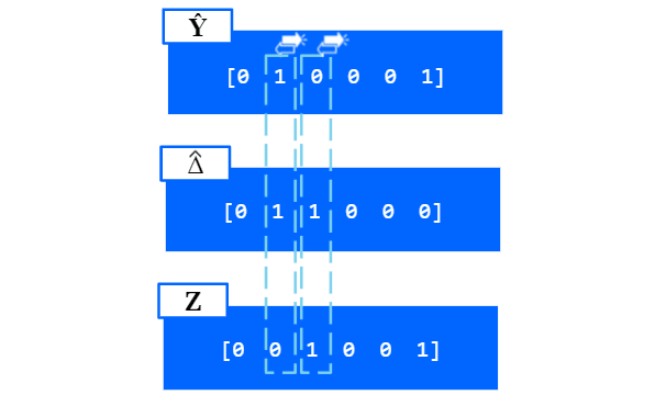
Finally, we can output our differentially private matrix, or vector in this case, Z.

This was a very technical, but also very minimalistic, introduction to the design of a differentially private algorithm. If you would like to read my entire thesis, you can reach out to me at mart.edva@gmail.com.
Finally, I hope that I’ve inspired some of you to pursue the algorithmic path throughout your education, which truly was my humble goal for this series of blog posts. I look forward to your feedback and a lively discussion in the comments!

Top comments (0)