Analyzing test data can seem much more difficult than numeric data, however the sklearn library provides useful
feature extraction tools that can transform any text data you may have into a numerical format. In addition to sklearn, the Natural Language Toolkit library provides many useful tools that can be vitally useful for further preprocessing textual data that is longer.
Below I will show how to use sklearn's CountVectorizor to convert reviews from a string to a matrix filled with numeric values for each review, plus some of the preprocessing tools, in order to predict the sentiment of IMDb reviews. The data set comes from kaggle where I have taken the training set and testing set, but omitted the validation set for simplicity.
The first step will be to load the data set into a pandas DataFrame and use df.info() to gain insights into the size of each dataset, the data types used and if there are any missing values.
import pandas as pd

df_train = pd.read_csv('imdb_review_sentiment_train.csv')
df_test = pd.read_csv('imdb_review_sentiment_test.csv')
df_train.head()
[output]
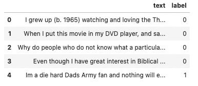
As you can see, the datasets contain two columns. One with the text from a review, and the other with the sentiment of the review under 'label'. Inspecting examples for each review revealed that a '0' indicates a negative review and a '1' indicates a positive one. There are also eight times as many reviews in our training set than our testing set, which should help the performance of our model.
df_train.info()
[output]

df_test.info()
[output]

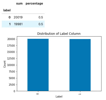
Our next step will be to checkout the distribution of our target variable to see if there is any class imbalance amongst the sentiments. To do this I have written a function that takes in a pandas Series and prints out a bar chart of the Series counts and returns a DataFrame presenting the Series' value_counts() output for the sum and percentages of the column.
# function to present and plot distribtuion of values in series
# automatically prints plot, summary df is returned to unpack and present
def summerize_value_counts(series):

    # extract name of series
    series_name = series.name

    # make dataframe to display value count sum and percentage for series
    series_count = series.value_counts().rename('sum')
    series_perc = series.value_counts(normalize=True).round(2).rename('percentage')
    series_values_df = pd.concat([series_count, series_perc], axis=1)

    # plot series distribution
    plot = series_values_df['sum'].plot(kind='bar', title=f'Distribution of {series_name.title()} Column',
                                 xlabel=f'{series_name.title()}', ylabel='Count');

    # rename df index to series name
    series_values_df.index.name = series_name
    series_values_df

    return series_values_df
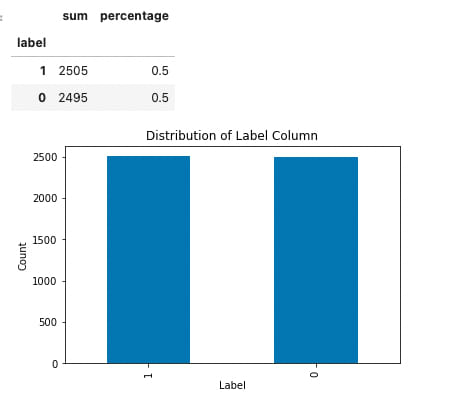
passing our label (sentiment) columns for both the training and testing datasets through shows us that each sentiment column is perfectly evenly distributed. We don't have to worry about class imbalance.
summerize_value_counts(df_train.label)
[output]
summerize_value_counts(df_test.label)
Next we will have to separate the data into our independent (reviews, or X variable) and dependent (sentiment, or y variable) variables for both the training and test sets. Additionally, let's convert all text values to lowercase to remove the effects of word case in our modeling.
# traning data
X_train = df_train.text.str.lower()
y_train = df_train.label

# testing data
X_test = df_test.text.str.lower()
y_test = df_test.label
However, our reviews are still in string format that the computer cannot understand with any context, so in order to turn each review into a numeric value we'll have to use sklearn's CountVectorizer. This will turn our column of reviews into a matrix with every word occuring in our dataset, or corpus in NLP nomenclature, becoming a column and every review, or document in NLP, becomes a row of zeros and ones. Intuitively, every word that appears in the review becomes a one in that column, with the others zeroed out.
Doing this is easy and only takes a few lines of code. After importing the CountVectorizer, simply initiate an instance object and fit and transform (so we have columns of words and rows of reviews) the training data and then transform the testing data.
from sklearn.feature_extraction.text import CountVectorizer

# initiate vectorizer
cv = CountVectorizer()

# fit and transform training data, than tranform testing data
X_train_cv = cv.fit_transform(X_train)
X_test_cv = cv.transform(X_test)
trying to view X_train shows it is a Compressed Sparse Row (csr) format that is not viewable with some code.
X_train_cv
[output]
<40000x92908 sparse matrix of type '<class 'numpy.int64'>'
    with 5463770 stored elements in Compressed Sparse Row format>
We can view it by converting X_train into an array and putting it into a DataFrame. We'll also apply thr .get_feature_names() method on our CountVectorizer object to label the columns.
df_cv = pd.DataFrame(X_train_cv.toarray(), columns=cv.get_feature_names())
df_cv.head()
df_cv.head()
[output]

This can be difficult to look at, so let's sort the dataframe, take the top five words and plot them.
df_cv.sum().sort_values(ascending=False)[:5].plot(kind='barh', title='Top Five Words',
                                                  xlabel='Word Count', ylabel='Words' );

With labeled data like this, it can also be useful to do these steps with the data split by sentiment to get a look and what words appear most per sentiment.
Now that we have our text data into numeric values, we are ready to model our data. I chose a Random Forrest classifier, but there are many binary classifiers out there to choose from.
We'll initiate an instance object of our model and then fit it with our new X_train_cv matrix and our normal y_train filled with each row's sentiment.
from sklearn.ensemble import RandomForestClassifier

forest_cv = RandomForestClassifier()
forest_cv.fit(X_train_cv, y_train)
using the models predict method and passing in our X_test_cv matrix we receive an array of predicted sentiment labels. passing this through sklearns accuracy_score() function gives us a score for our model.
from sklearn.metrics import accuracy_score

y_pred_cv = forest_cv.predict(X_test_cv)
accuracy_score(y_test, y_pred_cv)
[output]
0.8504
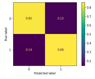
to dig a little deeper into our models performance, I also passed the model and testing data into sklearns plot_confusion_matrix() function to show the distribution of true/false positives and negatives. The bottom right corner (true 1, predicted 1) represents true positives while the top left corner (true 0, predicted 0) represents true negatives.
from sklearn.metrics import plot_confusion_matrix

plot_confusion_matrix(forest_cv, X_test_cv, y_test, normalize='true');
[output]
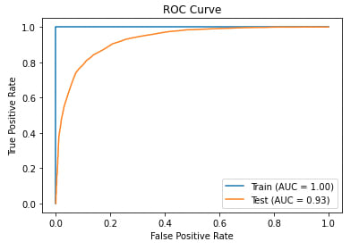
A further test of the model's performance is the ROC curve, which tests the power of the classifier as a function of false positives. The training data shows a perfect result, while the testing data shows very good results. The more area under the curve, the better the model performed.
from sklearn.metrics import plot_roc_curve
import matplotlib.pyplot as plt

# plot an ROC curve
fig, ax = plt.subplots()
plt.title('ROC Curve')
plot_roc_curve(forest_cv, X_train_cv, y_train, name='Train', ax=ax)
plot_roc_curve(forest_cv, X_test_cv, y_test, name='Test', ax=ax);
[output]
Although these reviews are not very long, they are still more words than tweets or headlines. This means it is worthwhile to explore some of NLTK's preprocessing functions that can be a useful way of reducing the effect of outlier words in text data to find underlying patterns in data.
To show a way of doing this, I will perform some preprocessing step by step on one review and then on the entire set of reviews.
# select a review as an example
example = X_train[3]
print(len(example.split()))
example
[output]
69
The first function is the RegexpTokenizer(), which is initialized with a regular expression to tokenize a string based on the regular expression passed through. A tokenized string becomes a list of substrings that have not been filtered out. The regular expression below will select only words beginning lower or uppercase letters and remove punctuation.
import nltk
from nltk.tokenize import RegexpTokenizer

regex_token = RegexpTokenizer(r"([a-zA-Z]+(?:’[a-z]+)?)")
after passing our example through the tokenize method of the RegexpTokenizer object, we see our example review has been converted to a list of substrings that cut the punctuation out of our review, which can be seen by the comma missing after 'movies' and the period after 'horror'
example_reg = regex_token.tokenize(example)
print(len(example_reg))
print(example_reg[:10])
print(example_reg[-1:])
[output]
69
['even', 'though', 'i', 'have', 'great', 'interest', 'in', 'biblical', 'movies', 'i']
['horror']
This is a good start, but there are many words like 'I', 'you', and 'do' that will weigh on our model due to their use in constructing sentences, but not reveal the contextual patterns we are looking for. In NLTK these are called 'stopwords' and removing them can further tokenize our text data to focus only on important strings. This can be done by iterating over our example review and only including words that are not in NLTK's English stop words.
from nltk.corpus import stopwords

sw = stopwords.words('english')
print(f'amount of english stopwords: {len(sw)}')
sw[:10]
[output]
amount of english stopwords: 179
['i', 'me', 'my', 'myself', 'we', 'our', 'ours', 'ourselves', 'you', "you're"]
# remove stopwords from example review
example_tokenized = [word for word in example_reg if word not in sw]
print(len(example_tokenized))
print(example_tokenized[:10])
[output]
33
['even', 'though', 'great', 'interest', 'biblical', 'movies', 'bored', 'death', 'every', 'minute']
This has cut our example review from 69 words to 33. Now that our review has been tokenized, let's explore ways to further cut the words in our data. We have already taken out punctuation and stopwords, but there are also words that are different to the computer that are effectively the same words, like 'movie' and 'movies'. As of now, the computer sees these two as completely different words, but it may help us find the underlying patterns for the sentiment of a text if we consider them the same. To do this, first we will use NLTK's pos_tag() function that will take our review, which is now a list of strings, and make each word a tuple with the words as the first element and the part of speech of the word as the second element.
from nltk import pos_tag

# pass part of speech to each word in the tokenized review
example_pos = pos_tag(example_tokenized)
example_pos[:10]
[output]
[('even', 'RB'),
 ('though', 'IN'),
 ('great', 'JJ'),
 ('interest', 'NN'),
 ('biblical', 'JJ'),
 ('movies', 'NNS'),
 ('bored', 'VBN'),
 ('death', 'NN'),
 ('every', 'DT'),
 ('minute', 'NN')]
These codes are hard to read, so let's make a list of the unique pos tags in our review and consult nltk.help.upenn_tagset() to get a description for each coded tag
unique_pos = set([x[1] for x in example_pos])

description = []
for pos in unique_pos:
    pos_described = nltk.help.upenn_tagset(pos)
    description.append(pos_described)
[output]
JJ: adjective or numeral, ordinal
    third ill-mannered pre-war regrettable oiled calamitous first separable
    ectoplasmic battery-powered participatory fourth still-to-be-named
    multilingual multi-disciplinary ...
RB: adverb
    occasionally unabatingly maddeningly adventurously professedly
    stirringly prominently technologically magisterially predominately
    swiftly fiscally pitilessly ...
VB: verb, base form
    ask assemble assess assign assume atone attention avoid bake balkanize
    bank begin behold believe bend benefit bevel beware bless boil bomb
    boost brace break bring broil brush build ...
IN: preposition or conjunction, subordinating
    astride among uppon whether out inside pro despite on by throughout
    below within for towards near behind atop around if like until below
    next into if beside ...
DT: determiner
    all an another any both del each either every half la many much nary
    neither no some such that the them these this those
NN: noun, common, singular or mass
    common-carrier cabbage knuckle-duster Casino afghan shed thermostat
    investment slide humour falloff slick wind hyena override subhumanity
    machinist ...
NNS: noun, common, plural
    undergraduates scotches bric-a-brac products bodyguards facets coasts
    divestitures storehouses designs clubs fragrances averages
    subjectivists apprehensions muses factory-jobs ...
VBG: verb, present participle or gerund
    telegraphing stirring focusing angering judging stalling lactating
    hankerin' alleging veering capping approaching traveling besieging
    encrypting interrupting erasing wincing ...
VBN: verb, past participle
    multihulled dilapidated aerosolized chaired languished panelized used
    experimented flourished imitated reunifed factored condensed sheared
    unsettled primed dubbed desired ...
The goal for these tuples is to find the stem of each word, the part responsible for its lexical meaning. This can be done with NLTK's WordNetLemmatizer, however we'll first have to convert the tag's pos_tag() gave us and then convert them into tags WordNetLemmatizer will recognize by using NLTK's wordnet. Below I have written a function that will do that by taking each word's pos_tag and converting it into a part of speech tag the lemmatizer will understand.
from nltk.corpus import wordnet

# This function gets the correct Part of Speech so the Lemmatizer can work
def get_wordnet_pos(treebank_tag):
    '''
    Translate nltk POS to wordnet tags
    '''
    if treebank_tag.startswith('J'):
        return wordnet.ADJ
    elif treebank_tag.startswith('V'):
        return wordnet.VERB
    elif treebank_tag.startswith('N'):
        return wordnet.NOUN
    elif treebank_tag.startswith('R'):
        return wordnet.ADV
    else:
        return wordnet.NOUN
Passing our list of tuples and putting each tag through our function returns a new list of tuples that is ready for our lemmatizer.
example_wordnet = [(word[0], get_wordnet_pos(word[1])) for word in example_pos]
example_wordnet[:10]
[output]
[('even', 'r'),
 ('though', 'n'),
 ('great', 'a'),
 ('interest', 'n'),
 ('biblical', 'a'),
 ('movies', 'n'),
 ('bored', 'v'),
 ('death', 'n'),
 ('every', 'n'),
 ('minute', 'n')]
Now to convert words to their stem, we'll initialize an instance object of our WordNetLemmatizer and pass each tuple through its lemmatize method.
from nltk.stem import WordNetLemmatizer

# initialize a lemmatizer
lemmatizer = WordNetLemmatizer()
Comparing our new list of strings we can see that 'movies' has been changed to 'movie' and 'bored' has been changed to 'bore'
# lemmatize each tuple to return a list a strings with some reducing towards their stem
example_lemmatized = [lemmatizer.lemmatize(word[0], word[1]) for word in example_wordnet]
example_lemmatized[:10]
[output]
['even',
 'though',
 'great',
 'interest',
 'biblical',
 'movie',
 'bore',
 'death',
 'every',
 'minute']
Finally, we can convert our review as a list of strings back into one string by joining our lemmetized version into a string with one space so words will be spaced.
example_rejoined = ' '.join(example_lemmatized)
example_rejoined
[output]
'even though great interest biblical movie bore death every minute movie everything bad movie long acting time joke script horrible get point mix story abraham noah together value time sanity stay away horror'
Comparing our final version to the original shows that our review has been shortened by 36 words, punctuation removed and some words reduced to their stem.
print(f'word count: {len(example.split())}')
print()
print(example)
print()
print(f'word count: {len(example_rejoined.split())}')
print()
print(example_rejoined)
[output]
word count: 69

even though i have great interest in biblical movies, i was bored to death every minute of the movie. everything is bad. the movie is too long, the acting is most of the time a joke and the script is horrible. i did not get the point in mixing the story about abraham and noah together. so if you value your time and sanity stay away from this horror.

word count: 33

even though great interest biblical movie bore death every minute movie everything bad movie long acting time joke script horrible get point mix story abraham noah together value time sanity stay away horror
Now let's put this whole process into a function, process our training data with that funciton and train a new random forrest with the preprocessed data.
def text_prep(text, sw):

    sw = stopwords.words('english')
    regex_token = RegexpTokenizer(r"([a-zA-Z]+(?:’[a-z]+)?)")
    text = regex_token.tokenize(text)
    text = [word for word in text]
    text = [word for word in text if word not in sw]
    text = pos_tag(text)
    text = [(word[0], get_wordnet_pos(word[1])) for word in text]
    lemmatizer = WordNetLemmatizer()
    text = [lemmatizer.lemmatize(word[0], word[1]) for word in text]
    return ' '.join(text)
def tokenize_vector(vectorizer, X_train, X_test):
#     sw = stopwords.words('english')

    X_train_tokenized = [text_prep(text, sw) for text in X_train]
    X_train_token_vec = vectorizer.fit_transform(X_train_tokenized)
    X_test_token_vec = vectorizer.transform(X_test)

    return X_train_token_vec, X_test_token_vec
cv_tok = CountVectorizer()

X_train_tokenized = [text_prep(text, sw) for text in X_train]

X_train_cv_tok = cv_tok.fit_transform(X_train_tokenized)
X_test_cv_tok = cv_tok.transform(X_test)

forest_cv_tok = RandomForestClassifier()

forest_cv_tok.fit(X_train_cv_tok, y_train)
y_pred_cv_tok = forest_cv_tok.predict(X_test_cv_tok)

accuracy_score(y_test, y_pred_cv_tok)
plot_confusion_matrix(forest_cv_tok, X_test_cv_tok, y_test, normalize='true');
[output]

# plot an ROC curve
fig, ax = plt.subplots()
plt.title('ROC Curve')
plot_roc_curve(forest_cv_tok, X_train_cv_tok, y_train, name='Train', ax=ax)
plot_roc_curve(forest_cv_tok, X_test_cv_tok, y_test, name='Test', ax=ax);
[output]
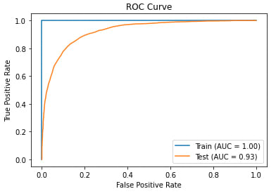
As you can see in this example, overall model accuracy has not changed, however with some trials not shown it improved and with more data to process these steps can work to find the patterns in textual data that will unlock growth as your models develop.

Top comments (0)