
Special numbers in numpy
The special value NaN actually means "not a number", it's a special number that is used for undefined math operations, such as 0/0 (division of anything else by zero makes a +/- infinity number accordingly). NaN and infinity are defined in the IEEE 754 standard of floating-point numbers.
NaN has a few special properties that aren't typical of other numbers. Any arithmetic operation involving a NaN will automatically make the result NaN (including with non-NaN numbers). Relational comparisons of NaN with any number will return False, including NaN == NaN. Consequentially, NaN != NaN returns True, and it's not possible testing normal relational operators whether a number is NaN. To get around this both python's math module and numpy define an isnan() function for testing if a number is NaN.
In [7]: math.isnan(1)
Out[7]: False

In [9]: math.isnan(math.nan)
Out[9]: True

In [14]: np.isnan(np.array(0)/0)
<ipython-input-14-b138b724fd93>:1: RuntimeWarning: invalid value encountered in true_divide
  np.isnan(np.array(0)/0)
Out[14]: True

In [16]: np.isnan(np.nan)
Out[16]: True
In addition to the above, both modules also have isfinite() and isinf() functions that test if a number is finite or infinity, respectively. NaN is neither finite nor infinite.
Convenience functions that remove NaN values from arrays before operating on them are nansum(), nanmax(), nanmin(), nanargmax(), nanargmin(). (argmin and argmax funcions take the minimum/maximum values and return the indices where they are attained.)
>>> x = np.arange(10.)
>>> x[3] = np.nan
>>> x.sum()
nan
>>> np.nansum(x)
42.0
An explanation of floating point numbers follow. It will likely be most appreciated by numpy users interfacing with C code. It would be helpful to know how floating-point numbers are represented in memory.
A floating point format consists of a base aka radix, precision and range. Since we are concerned how the numbers are represented in computer memory, the base is almost always 2.
All floating point formats are made by IEEE. You can't make your own formats.
The range, emax and emin are the maximum and minimum exponents this format can represent. emin = 1 - emax.
The precision p, is how many digits this format can store. It is specified as a binary number not a decimal number, so a float32 can store about 7 decimal digits which translates to 23 binary digits, a float64 can store about 15 decimal digits which translates to 52 binary digits.
Emphasis must be put in the use of the word format. The above information is only contained in foating point formats like float32, double, etc, not the numbers themselves.
As for what floating point numbers contain, assuming you have the floating point format for it, it also has fields stored as binary digits.
First there is ovbiously the sign, which is one bit which determines if the number is negative or positive. Note that IEEE has two different zeroes: +0 and -0, but virtually all languages treat them as equal.
Then there is the exponent q, the field where the binary exponent of a binary number is stored in. To be representable, the exponent plus the precision (minus 1) needs to be between the range, [emin..emax] inclusive.
The mantissa aka significand of a floating point number containts the digits of a number in the base. Rememher that the base is almost always 2 which means the mantissa will be specified as a fractional binary number such as 0.10011 or something like that.
For example, 85.125 (a floating point number) = 1010101.001b (.001b corresponding to 1/8 in decimal) = 1.010101001b (mantissa) x 2^6 (binary scientific notation, the 'b' at the end of the number is one I put there to symbolize "binary number"). The 6 is stored in the exponent. Actually, first the 6 is added to some integer called a bias which effectively increases it by a fixed amount into an unsigned number, and then the result is stored in the exponent. For example, float32 has 8-bit exponents and the bias is 127, float64 has 11-bit exponents and the bias is 1023.
The reason why bias is necessary is because it is easier to compare unsigned exponents to compare floating point numbers, than to compare signed exponents which are represented very differently than signed numbers (the last bit is always set for negative numbers, and the bits are OR'd and AND'd in the reverse order if you count from -1..-127 versus 1..127, and other things to wrap your head around. They won't be expounded upon in this post). So it's just easier to compare floating point numbers if the exponent is internally represented as an unsigned number.
All in all, think of floating point numbers like a struct:
number
|
|- sign
|
|- exponent
|
|- mantissa
|
|- format
        |
        |- base
        |
        |- precision
        |
        |- range
Numerical exceptions
The possible numerical exceptions available in numpy are overflow, underflow, invalid argument and division by zero. Now, invalid argument exception is not the typical kind of bad parameters you pass to functions, it specifically means passing arguments outside the domain of the function, like any argument to arcsin() (inverse sine) or arccos() outside the range [-1..1].
You have the option of ignoring the error, printing a warning or error, calling an error callback, or logging the error. Specifically, these can be passed as values (of keyword args) to np.seterr():
- 'ignore' : Take no action when the exception occurs.
- 'warn' : Print a RuntimeWarning (via the Python warnings module).
- 'raise' : Raise a FloatingPointError.
- 'call' : Call a function specified using the seterrcall function.
- 'print' : Print a warning directly to stdout.
- 'log' : Record error in a Log object specified by seterrcall.
These are the available keyword argument names to np.seterr():
- all : apply to all numeric exceptions
- invalid : when NaNs are generated
- divide : divide by zero (for integers as well!)
- overflow : floating point overflows
- underflow : floating point underflows
>>> oldsettings = np.seterr(all='warn')
>>> np.zeros(5,dtype=np.float32)/0.
invalid value encountered in divide
>>> j = np.seterr(under='ignore')
>>> np.array([1.e-100])**10
>>> j = np.seterr(invalid='raise')
>>> np.sqrt(np.array([-1.]))
FloatingPointError: invalid value encountered in sqrt
>>> def errorhandler(errstr, errflag):
...      print("saw an error!")
>>> np.seterrcall(errorhandler)
<function err_handler at 0x...>
>>> j = np.seterr(all='call')
>>> np.zeros(5, dtype=np.int32)/0
FloatingPointError: invalid value encountered in divide
saw an error!
>>> j = np.seterr(**oldsettings) # restore previous
...                              # error-handling settings
Byte swapping
As I have shown in Part 3, numpy can emulate different byte orders. In order to fully appreciate this feature, it is necesarry to understand what byte order is.
An introdcution to byte order
If you're reading this article right now, you're either reading it on PC, whose processor uses little endian bytes, or on a mobile device, whose processor can use little or big endian bytes but the underlying OS is most likely using little endian anyway.
Personal computers use an x86-compatible processor such as Intel or AMD. These can only do little endian. On the other hand, phones and tables have ARM-based processors in them, and the ARM architecture can run in little endian or big endian mode. However, most mobile operating systems like Android and iOS choose to run it in little endian. Thus, the vast majority of systems you see will run in little endian mode.
As for what little-endian mode is: Suppose you have a 32-bit integer, like 20201403 (which has the binary representation (0000 0001 ___ 0011 0100 ___ 0011 1111 ___ 1011 1011). This has four bytes, which I separated with underscores. Now the most significant bit is the zero because it's at the left of the number, and the least significant bit is the one, because it's the right-most digit. Then a big endian system will write the binary numbers in its memory from left to right, like I just did. In fact, the way of writing big endian numbers is in the same direction people write them on paper.
Now little endian systems write the binary digits in it's memory from right to left, like certain Eastern languages. That means the above number will be stored on a little endian system (the vast majority of systems in production use in the world) as 1101 1101 ___ 1111 1100 ___ 0010 1100 ___ 1000 0000. As you can see, I flipped the number around, reversed it. The most significant bit (MSB) is now at the right and the least significant bit (LSB) is at the left. On a little endian system this will correctly store the number as 20201403.
On a big endian system this number will be interpreted completely wrong (3724291200 in this case). That is why it's imporatnt to keep track of the positions of the MSB and LSB in a sequence of bytes.
We say that little endian has a left MSB, right LSB, and that big endian has a right MSB, left LSB.
But since every system you're probably going to use is little endian, why do we have big endian in the first place? Well, to transmit these items and data across the network, they have to be converted to big endian first and then back into whatever byte order the target computer is using. Networks, and transmission of data across IP addresses uses the big endian format. This allows all systems to understand the order the data is in, instead of simply transmitting it with whichever endian the host is using.
For all endians, only bytes are swapped. Bits of a byte are never swapped.
Byte order as used in numpy and python
At first glance at numpy output, it may look like there is no visible difference between using big endian or little endian. That's because python and numpy handle these differences internally. Bare-bones languages like C and C++ do not handle this difference so it is easier to spot data in the wrong byte order if it looks like a nonsensical value.
In [1]: big_end_arr = np.array([4, 5],dtype='>i2')         # '>' is big endian

In [2]: big_end_arr
Out[2]: array([4, 5], dtype=int16)

In [3]: little_end_arr = np.array([4, 5],dtype='<i2')     # '<' is little endian

In [4]: little_end_arr
Out[4]: array([4, 5], dtype=int16)
In this second example, I demonstrate a case where byte order of the array matters:
In [1]: buffer = bytearray([0,1,3,2])                    # bytearray is an array of 8-bit integers (bytes)

In [2]: np.ndarray(shape=(2,),dtype='>i2', buffer=buffer)          # big endian
Out[2]: array([  1, 770], dtype=int16)

In [3]: np.ndarray(shape=(2,),dtype='<i2', buffer=buffer)         # little endian
Out[3]: array([256, 515], dtype=int16)
The big endian array uses the 8-bit integers 0 and 1 to construct the first element 1, the second element 770 is constructed with the elements 3 and 2.
On the other hand, the little endian array uses the integers 1 and 0 to construct the first element 256, and the elements 2 and 3 to construct the second element 515.
The reason only two integers are being swapped at a time is because this is an array of 16-bit integers. If it was an array of 32-bit integers, then the big endian array would be size 1x1, the element composed of the numbers 0, 1, 3, 2 and the little endian array would be size 1x1, the element composed of the numbers 2, 3, 1, 0.
Swapping the byte order
Numpy makes it easy for you to change the underlying byte order without running into the above problem. dtypes provides a method called newbyteorder() that flips the endianness of the dtype. You also need to call <some-array>.byteswap() to flip the bytes in all the elements. These two functions work independently and neither is called by the other, so you must call both of them, otherwise the resulting elements will be nonsensical.
Record arrays
recarrays allow you to access fields of a struct array by attribute instead of just by index. They are created by calling np.rec.array():
>>> recordarr = np.rec.array([(1, 2., 'Hello'), (2, 3., "World")],
...                    dtype=[('foo', 'i4'),('bar', 'f4'), ('baz', 'S10')])
>>> recordarr.bar
array([ 2.,  3.], dtype=float32)
>>> recordarr[1:2]
rec.array([(2, 3., b'World')],
      dtype=[('foo', '<i4'), ('bar', '<f4'), ('baz', 'S10')])
>>> recordarr[1:2].foo
array([2], dtype=int32)
>>> recordarr.foo[1:2]
array([2], dtype=int32)
>>> recordarr[1].baz
b'World'
You can convert a normal array to a recarry by passing it to np.rec.array(). But if you just want a shallow copy (view) of a struct array, then use something like this. It makes use of the dtype((base_dtype, new_dtype)) construct.
>>> arr = np.array([(1, 2., 'Hello'), (2, 3., "World")],
...                dtype=[('foo', 'i4'),('bar', 'f4'), ('baz', 'a10')])
>>> recordarr = arr.view(dtype=np.dtype((np.record, arr.dtype)),
...                      type=np.recarray)
>>> recordarr = arr.view(np.recarray)       # This also works
>>> recordarr.dtype
dtype((numpy.record, [('foo', '<i4'), ('bar', '<f4'), ('baz', 'S10')]))
This is how you get a view of a normal/struct array from a recarray:
arr = recordarr.view(recordarr.dtype.fields or recordarr.dtype, np.ndarray)
dtype.fields only exists if dtype is a struct array.
Nifty examples that use numpy
Most of these are from numpy docs, kudos to them.
# Searching the maximum value of a time-dependent series
>>> time = np.linspace(20, 145, 5)                 # time scale
>>> data = np.sin(np.arange(20)).reshape(5,4)      # 4 time-dependent series
>>> time
array([  20.  ,   51.25,   82.5 ,  113.75,  145.  ])
>>> data
array([[ 0.        ,  0.84147098,  0.90929743,  0.14112001],
       [-0.7568025 , -0.95892427, -0.2794155 ,  0.6569866 ],
       [ 0.98935825,  0.41211849, -0.54402111, -0.99999021],
       [-0.53657292,  0.42016704,  0.99060736,  0.65028784],
       [-0.28790332, -0.96139749, -0.75098725,  0.14987721]])
>>>
>>> ind = data.argmax(axis=0)                  # index of the maxima for each series
>>> ind
array([2, 0, 3, 1])
>>>
>>> time_max = time[ind]                       # times corresponding to the maxima
>>>
>>> data_max = data[ind, range(data.shape[1])] # => data[ind[0],0], data[ind[1],1]...
>>>
>>> time_max
array([  82.5 ,   20.  ,  113.75,   51.25])
>>> data_max
array([ 0.98935825,  0.84147098,  0.99060736,  0.6569866 ])
>>>
>>> np.all(data_max == data.max(axis=0))
True
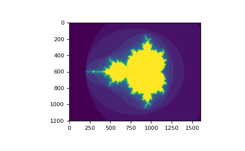
# Using boolean indexing to create an image of the Mandelbrot set.
# This example requires you have the matplotlib package installed.
In [26]: import numpy as np
    ...: import matplotlib.pyplot as plt
    ...: def mandelbrot( h,w, maxit=20 ):
    ...:     """Returns an image of the Mandelbrot fractal of size (h,w)."""
    ...:     y,x = np.ogrid[ -1.4:1.4:h*1j, -2:0.8:w*1j ]
    ...:     c = x+y*1j
    ...:     z = c
    ...:     divtime = maxit + np.zeros(z.shape, dtype=int)
    ...:
    ...:     for i in range(maxit):
    ...:         z = z**2 + c
    ...:         diverge = z*np.conj(z) > 2**2            # who is diverging
    ...:         div_now = diverge & (divtime==maxit)  # who is diverging now
    ...:         divtime[div_now] = i                  # note when
    ...:         z[diverge] = 2                        # avoid diverging too much
    ...:
    ...:     return divtime
    ...: plt.imshow(mandelbrot(400,400))
    ...: plt.show()
    ...:
# Histogram plot showcasing numpy's random number generator.
>>> import numpy as np
>>> import matplotlib.pyplot as plt
# Build a vector of 10000 normal deviates with variance 0.5^2 and mean 2
>>> mu, sigma = 2, 0.5
>>> v = np.random.normal(mu,sigma,10000)
# Plot a normalized histogram with 50 bins
>>> plt.hist(v, bins=50, density=1)       # matplotlib version (plot)
>>> plt.show()
# The same plot but with bins computed by numpy instead of matplotlib
>>> (n, bins) = np.histogram(v, bins=50, density=True)  # NumPy version (no plot)
>>> plt.plot(.5*(bins[1:]+bins[:-1]), n)
>>> plt.show()
This is matplotlib's histogram:

And this is the histogram made by numpy:

And we're done
This wraps up the numpy series. Thank you for reading. 🙌
Much material was sourced from the numpy manual.
If you see any errors here (and previous posts did contain incorrect information), please let me know so I can fix them.

Top comments (0)