
Introduction
Data modeling is about how the tables of Power BI gets organized and linked with other tables so it can properly do the work. In this article I will be going through the basic building blocks of Power BI data modeling - SQL-style joins, relationships, fact vs dimension tables, schema patterns, and the common mistakes I see people make all the time. I’ll try to keep it practical in the form of examples and give you real guidance on where to click in the Power BI interface.
Part 1: What Is Data Modeling?
Data modeling is about determining how you structure your tables and how they communicate with one another. In Power BI, your data model is everything — the tables, relationships between them, and calculated columns and measures you build on top.
Part 2: SQL Joins — Combining Data Before It Hits the Model
Before your data even makes it into the Power BI model, you often need to combine tables from different sources. That's where joins come in.

A join is like asking, “Every row in this table, which rows in this other table match up?” The answer varies depending on what type of join you choose. A common catch for beginners is the fact that joins happen in Power Query Editor the transformation layer and not the model itself. You're literally smashing tables together before they load.
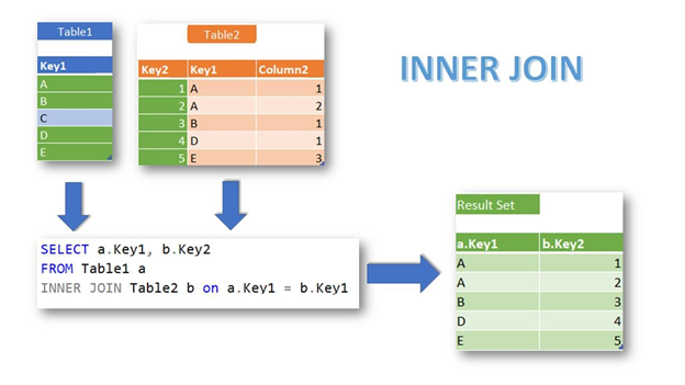
2.1 INNER JOIN
This one is the strictest. It will only show you rows when both tables match. No match? That row gets tossed.
Say you have an Orders table and Customers table. When you INNER JOIN on CustomerID, the data that appears from customers you've already recorded to your Customers table is only for those customers currently in it. Got an order from customer C3 (your order, but C3 isn't in your customer list)? Gone.
Orders Table Customers Table
┌──────────┬────────┐ ┌──────────┬──────────┐
│ OrderID │ CustID │ │ CustID │ Name │
├──────────┼────────┤ ├──────────┼──────────┤
│ 1001 │ C1 │ │ C1 │ Alice │
│ 1002 │ C2 │ │ C2 │ Bob │
│ 1003 │ C3 │ │ C4 │ Diana │
│ 1004 │ C5 │ │ C5 │ Eve │
└──────────┴────────┘ └──────────┴──────────┘
INNER JOIN Result (on CustID):
┌──────────┬────────┬──────────┐
│ OrderID │ CustID │ Name │
├──────────┼────────┼──────────┤
│ 1001 │ C1 │ Alice │
│ 1002 │ C2 │ Bob │
│ 1004 │ C5 │ Eve │
└──────────┴────────┴──────────┘
→ Order 1003 (C3) is dropped: no match in Customers.
→ Customer C4 (Diana) is dropped: no matching Order.
plaintext
2.2 LEFT (OUTER) JOIN
This is the join I use most. You keep every row from the left table, and if there's a match in the right table, great — those columns get filled in. If not, you get nulls, but the row stays.
Basically a LEFT JOIN flipped. Everything from the right table stays, with matching rows from the left traveling along. Unmatched left-side stuff appears as null. If you needed to see all your customers — even those who’d never bought anything — you would use this. Diana would show up with null for OrderID. As it stands now, most analysts I know just swap the table order and use a LEFT JOIN. Same outcome, easier to keep track of.
LEFT JOIN Result (Orders LEFT JOIN Customers on CustID):

┌──────────┬────────┬──────────┐
│ OrderID  │ CustID │ Name     │
├──────────┼────────┼──────────┤
│ 1001     │ C1     │ Alice    │
│ 1002     │ C2     │ Bob      │
│ 1003     │ C3     │ null     │  ← No match, but order sticks around
│ 1004     │ C5     │ Eve      │
└──────────┴────────┴──────────┘
→ All 4 orders are preserved.  Diana (C4) does not show up, because she has no orders.
plaintext
This is your go-to when the left table is the important one and you want to enrich it with extra info from somewhere else.
2.3 RIGHT (OUTER) JOIN
RIGHT JOIN Result (Orders RIGHT JOIN Customers on CustID):
┌──────────┬────────┬──────────┐
│ OrderID  │ CustID │ Name     │
├──────────┼────────┼──────────┤
│ 1001     │ C1     │ Alice    │
│ 1002     │ C2     │ Bob      │
│ null     │ C4     │ Diana    │  ← No order, but she stays
│ 1004     │ C5     │ Eve      │
└──────────┴────────┴──────────┘
→ Order 1003 (C3) is dropped because C3 is does not exist in Customers.
plaintext
2.4 FULL OUTER JOIN
The "keep everything" option. Every row from both tables comes into the output. Columns merge where there is a match between the rows. Where there isn’t, you get nulls on whichever side is missing. This is a lot easier when it comes to data reconciliation, when you’re trying to find what is in Table A and what is not in Table B or vice versa.
FULL OUTER JOIN Result:
┌──────────┬────────┬──────────┐
│ OrderID  │ CustID │ Name     │
├──────────┼────────┼──────────┤
│ 1001     │ C1     │ Alice    │
│ 1002     │ C2     │ Bob      │
│ 1003     │ C3     │ null     │  ← Order with no customer
│ null     │ C4     │ Diana    │  ← Customer with no order
│ 1004     │ C5     │ Eve      │
└──────────┴────────┴──────────┘
→ Nothing gets dropped. Both orphaned sides are preserved.
plaintext
I mostly pull this out during data quality audits, or when I'm first exploring a new dataset and want to see what matches up and what doesn't.

2.5 LEFT ANTI JOIN
For data validation, I'm a fan of this one personally. It only gives you the left-table rows that do not have a match on the right. It is kind of the opposite of an INNER JOIN. Looking for orders that refer to a customer ID that is nonexistent? Left anti join. Boom — orphaned records.
LEFT ANTI JOIN Result:
┌──────────┬────────┐
│ OrderID  │ CustID │
├──────────┼────────┤
│ 1003     │ C3     │  ← This order has no matching customer
└──────────┴────────┘
Super useful for catching data integrity problems early.
2.6 RIGHT ANTI JOIN
Same idea, other direction. Gives you rows from the right table that have no match in the left. Classic use case: identify customers who have never placed a single order.
RIGHT ANTI JOIN Result:
┌────────┬──────────┐
│ CustID │ Name     │
├────────┼──────────┤
│ C4     │ Diana    │  ← Never ordered anything
└────────┴──────────┘
Used for identifying inactive customers, unused products, or anything that should be connected but isn't.
2.7 How to Actually Do Joins in Power BI
All of this happens in Power Query Editor, through the Merge Queries feature. Here's how to do it:
Step 1: Open Power BI Desktop. Hit Transform Data on the Home ribbon — that drops you into Power Query Editor.
Step 2: In the Queries pane on the left, click the table you want as your "left" table.
Step 3: On the Home ribbon inside Power Query, click Merge Queries.
Step 4: The Merge dialog will pop up. Your left table is pre-selected at the top. Pick your right table from the dropdown below. Click the matching column in both table previews — like CustID in each. Then, at the bottom, choose your Join Kind: Inner, Left Outer, Right Outer, Full Outer, Left Anti, or Right Anti.
Step 5: Click OK. A new column shows up containing nested tables — that's the merged data.
Step 6: Click the expand icon (those little arrows ↔) on the new column header and pick which columns from the right table you want to bring in.
Step 7: Hit Close & Apply and the merged result loads into your model.
Part 3: Power BI Relationships
Here's where things differ from joins in an important way. Joins combine two tables into one. Relationships keep the tables separate but create a logical link between them inside the model. They tell Power BI how to filter across tables and aggregate data without actually merging anything.
So: joins happen during data loading (in Power Query). Relationships exist within the model, after the data's already loaded. This distinction matters.
3.1 Cardinality
Cardinality shows how many rows on one side can match rows on the other."
One-to-Many (1:M) — This Is What You Want
Think of it this way: one customer can have many orders, but each order belongs to him only.
Customers (1 side)          Orders (Many side)
┌────────┬────────┐         ┌──────────┬────────┬────────┐
│ CustID │ Name   │         │ OrderID  │ CustID │ Amount │
├────────┼────────┤         ├──────────┼────────┼────────┤
│ C1     │ Alice  │───1:M──▶│ 1001     │ C1     │ 50     │
│        │        │         │ 1005     │ C1     │ 120    │
│ C2     │ Bob    │───1:M──▶│ 1002     │ C2     │ 80     │
└────────┴────────┘         └──────────┴────────┴────────┘
Why is this the gold standard? Because filters flow cleanly. Choose “Alice” in a slicer and Power BI identifies and displays which orders to show. Aggregations will work here.
Many-to-Many (M:M)
This occurs when neither table has unique values in the join column. Multiple rows match multiple rows on both sides.
A common example would be students and courses — each student takes multiple courses, each course has several students. If you link these directly without a bridge table, you’ve got an M:M relationship on your hands.
The problem? Filters can get weird. You might have double counting or totals that are larger than they should be. Power BI technically does allow M:M relationships, but in my experience, they're generally a sign that there isn't a bridge table in between.
One-to-One (1:1)
Each row exactly corresponds to one row in the other table. Both sides have unique values.
A lot of times this can be seen in situations where a specific table may have been split into two for the sake of organization.
3.2 Cross-Filter Direction
- Single Direction (typically the right choice) Filters from the "one" side to the "many" side only like a one way.
Customers ──filter──▶ Orders. (Select a customer → their orders are filtered).
Orders ──X──▶ Customers. (Choose an order → doesn’t filter the Customers table)
This keeps things predictable. Dimension tables filter fact tables, not the other way around. Exactly what you want for most reports.

#### Bidirectional
Filters travel both ways. Selecting something in either table filters the other.
plaintext
Customers ◀──filter──▶ Orders
I’d say use this sparingly. There are genuine scenarios — certain M:M bridge table setups need it — but when people start flipping everything to bidirectional, things get messy. Performance takes a hit, and you can end up with filter behavior that nobody on your team can explain.

My rule of thumb: start with single direction. Only switch to bidirectional when you've got a concrete reason and you've tested the impact.

---

### 3.3 Active vs. Inactive Relationships
Power BI only lets you have **one active relationship** between any two tables at a time. If you've got multiple connections between the same pair of tables, pick one as active — the rest as inactive.

Here is where this comes up constantly. Your `Sales` table has `OrderDate`, `ShipDate`, and maybe `DeliveryDate`. All three should connect to your `Calendar` table. But only one relationship can be active at a time.
plaintext
Calendar (Date)
│
├── Active Relationship ──── Sales[OrderDate]
│
└── Inactive Relationship ─ ─ ─ SalesShipDate
Active relationship is the default function used by DAX. If you need the inactive one, you write USERELATIONSHIP:
Ship Date Sales =
CALCULATE(
    SUM(Sales[Amount]),
    USERELATIONSHIP(Sales[ShipDate], Calendar[Date])
)
Not the best solution, but it works. In my dimensions role-playing later on, I'll discuss some possible alternate methods.
3.4 Creating relationships-step by step
There are three methods for doing that.
Method 1: Drag and Drop in Model View
Click the Model View icon in your left sidebar (the one that looks like three boxes) and you will actually see how they are connected together. You will notice all your tables arranged. You just tap one column in one table and drag it to the other corresponding column. Power BI auto-determines the cardinality and filter direction — so just click on the line twice to adjust those settings.
Method 2: Manage Relationships Dialog
Redirect to Home (or Modeling) ribbon → Manage Relationships. Click New, select your tables and columns from the dropdowns, set cardinality, filter direction, select if it's active, and hit the OK button.
Method 3: Let Power BI Auto-Detect
Once you load the data, Power BI will then try to guess some relationships based on column names and what data types you have. It does an okay job for stuff, but I always check what it generates. Go to Manage Relationships and check. I've watched auto-detect build quite dubious relationships.
Part 4: Joins vs. Relationships — What Is the Difference?
This mystifies people who are just getting started, so just a couple words:

| Aspect | Joins (Power Query) | Relationships (Model) |
|---|---|---|
| Where | Power Query Editor | Model View / Manage Relationships |
| When | During data loading | After data is in the model |
| What happens | Tables physically merge into one | Tables stay separate, linked logically |
| Row count | Can change (more or fewer rows) | Tables keep their original row counts |
| When to use | Enriching or cleaning data | Enabling cross-table filtering and aggregation |
| Performance | Makes tables bigger | VertiPaq handles it efficiently |
| DAX | Merged columns are all in one table | Uses RELATED/RELATEDTABLE to traverse |
My general rule: Use joins (Merge in Power Query) when you need to physically combine or clean stuff — adding a lookup value or deduplicating. Use relationships for pretty much everything else. Keeping tables separate and letting Power BI handle the filtering is always the better approach.
Part 5: Fact Tables vs. Dimension Tables
If there's one concept that makes everything click, it's understanding the difference between facts and dimensions. This is the foundation.
Fact Tables
These hold the events — the things that happened. A sale, a shipment, a website click, a support ticket. Each row is a transaction.
What makes a fact table a fact table:
- It has measures — numbers you want to add up (revenue, quantity, cost, duration)
- It has foreign keys — pointers to dimension tables (CustomerID, ProductID, DateKey)
- It's tall — lots of rows, not too many columns
- It grows — new transactions keep getting added
Think: Sales, Orders, WebClicks, SupportTickets, Shipments.
Dimension Tables
These provide the context — the who, what, where, when, and why behind your transactions.
What makes a dimension table a dimension table:
- It has descriptive columns — names, categories, regions, dates
- It has a primary key — a unique identifier for each row
- It's wide — many columns, relatively fewer rows
- It changes slowly — a customer's name or address doesn't change every day
Think: Customers, Products, Calendar, Geography, Employees, Stores.
How They Fit Together
┌──────────────┐     ┌──────────────────────────────┐     ┌──────────────┐
│  Customers   │     │         Sales (Fact)          │     │   Products   │
│  (Dimension) │     │                               │     │  (Dimension) │
├──────────────┤     ├──────────────────────────────┤     ├──────────────┤
│ *CustomerID  │◀─1:M│ SaleID                        │M:1─▶│ *ProductID   │
│  Name        │     │ CustomerID (FK)               │     │  ProductName │
│  City        │     │ ProductID (FK)                │     │  Category    │
│  Segment     │     │ DateKey (FK)                  │     │  Price       │
└──────────────┘     │ Quantity                      │     └──────────────┘
                     │ Amount                        │
                     └──────────────────────────────┘
                                   │
                                  M:1
                                   │
                              ┌─────────┐
                              │Calendar │
                              │(Dim)    │
                              ├─────────┤
                              │*Date    │
                              │ Month   │
                              │ Quarter │
                              │ Year    │
                              └─────────┘
The asterisk identifies the primary key. Filters move from the dimension tables (the "one" side) to the fact table (the "many" side). Choose a customer, a product, or a date — and the sales figures update accordingly. That's the whole magic trick.
Part 6: Schema Designs
Schema is just a word for the overall shape of your model — how you've arranged your fact and dimension tables.
6.1 Star Schema
If you take one thing away from this entire article, let it be this: use of a star schema. It's what Power BI was designed for.
The idea is simple. You’ve got a fact table in the center, and your dimension tables connect to it directly — like points on a star.

                    ┌────────────┐
                    │  Calendar  │
                    └──────┬─────┘
                           │
┌────────────┐    ┌────────┴────────┐    ┌────────────┐
│ Customers  ├────┤   Sales (Fact)  ├────┤  Products  │
└────────────┘    └────────┬────────┘    └────────────┘
                           │
                    ┌──────┴─────┐
                    │   Stores   │
                    └────────────┘
Every dimension goes directly to the fact table. The dimensions themselves are denormalized, so you group all the descriptive properties into a single table, even if there’s some duplication. You maintain a ProductName, a SubCategory, a Category, and a Department in one table, even though that hierarchy technically could be normalized into separate tables. Why bother with the redundancy? Because it's worth it. Power BI's VertiPaq engine is optimized for exactly that kind of pattern. Filters from dimension to fact — no detours. DAX behaves predictably. Report writers can uncover what they need without detective work. In practically every project, I rely on star schemas. It should be your default.
6.2 Snowflake Schema
A snowflake schema is what happens when you take a star schema and normalize the dimensions — splitting them into chains of sub-tables.
┌──────────────┐    ┌──────────────┐    ┌──────────────────┐
│  Department  ├────┤  Category    ├────┤    Products      │
└──────────────┘    └──────────────┘    └────────┬─────────┘
                                                 │
                                        ┌────────┴────────┐
                                        │  Sales (Fact)   │
                                        └────────┬────────┘
                                                 │
                                          ┌──────┴─────┐
                                          │  Calendar  │
                                          └────────────┘
While one Products table might have everything, now you have Products → Category → Department as separate tables in a chain. If this is a traditional SQL data warehouse, it's going to save storage space. But in Power BI? VertiPaq already compresses data incredibly well, so those storage savings are basically meaningless. Meanwhile, you’ve added extra problems for filters to travel through, made writing DAX hard, and confused anyone who tries to build a report. My advice: if the source data that you’re using is snowflaked (and that is often the case when it comes from enterprise data warehouses), flatten those dimension chains before you load them in Power Query. Merge the sub-tables back together. Turn it into a star.

6.3 Flat Table
This is the approach of "dump everything into one giant table." That is — facts, dimensions, all of it — one wide table with no associations in it, because there’s nothing to connect to.
┌─────────────────────────────────────────────────────────┐
│                   FlatSalesTable                        │
├─────────────────────────────────────────────────────────┤
│ SaleID │ Date │ CustomerName │ City │ ProductName │ ... │
│ Amount │ Quantity │ Category │ Segment │ StoreName │ ... │
└─────────────────────────────────────────────────────────┘
Look, we've all done this. You export something out of Excel and load it directly into Power BI and begin building visuals. For a quick personal analysis with a few hundred rows, it works, for sure.
But the second you scale up, things unravel. Every single row has repeat customer names and addresses. The file balloons in size. Compression suffers. DAX becomes quirky since a measure is hard to tell apart from a descriptive attribute. And heaven help you if you ever needed to update a customer address — you'd have to change it on maybe thousands of rows.
Flat tables make analysis easy to toss. If you need to separate your facts apart from your dimensions for anything else, take the time to do so.
6.4 Quick comparison
| Star Schema | Snowflake Schema | Flat Table | |
|---|---|---|---|
| Complexity | Low | Medium-High | Lowest |
| Power BI Performance | Best | Decent (extra hops) | Poor at scale |
| Data redundancy | Some (in dimensions) | Low | Very high |
| DAX friendliness | Very friendly | Trickier (multi-hop) | Unpredictable |
| Scalability | Excellent | Good | Poor |
| My Recommendation | default choice | Flatten it first | Small stuff only |

Part 7: Role-Playing Dimensions
Here’s one scenario that crops up all the time. You’ve got a Calendar table, and your Sales fact table has a bunch of date columns — OrderDate, ShipDate, DeliveryDate. All three logically connect to the same Calendar table, but they each contribute a disparate analytical perspective. This is a role-playing dimension. There is one dimension table and multiple hats on.
When you need ship date analysis, employ USERELATIONSHIP in DAX:
Shipped Amount =
CALCULATE(
    SUM(Sales[Amount]),
    USERELATIONSHIP(Sales[ShipDate], Calendar[Date])
)
It’s something tidy too. One calendar to follow. On the downside, report writers have to be informed that they get USERELATIONSHIP and only the active relationship can work by default.
Option B: Duplicate Calendar Table
Make separate calendar tables in Power Query — OrderCalendar, ShipCalendar, DeliveryCalendar — with its own active relationship to the date column. Also, more tables in the model. I have come to realize with every relationship in operation, you do not use USERELATIONSHIP, you can drop independent slicers for each date role without DAX gymnastics. When secondary date roles are seldom discussed in reports I opt for Option A. If stakeholders always have to slice by ship date and delivery date as well as by order date, Option B saves a lot of headaches.
Part 8: Common Data Modeling Mistakes and How to Correct Them
Let me take you through the problems I encounter most frequently.
Ambiguous Relationships
What you will see: A mistake regarding the presence of a relationship between tables, or as in “ambiguous paths.”
What you missed: You have multiple active paths between two tables, and Power BI cannot determine which relationship to use.
The fix: That any two tables will connect only one active relationship. And put the extras on dormant, USE USERELATIONSHIP if you need them.
Circular Dependencies
What you’ll see: Power BI does not want to form a relationship, and cautions against circular dependencies.
What went wrong: Your relationships build a loop — A connects to B, B connects to C, C connects back to A. Power BI doesn't know which way filters flow round the round.
The fix: Break the loop. Typically this involves cutting out a repetitive relation or adding the tables together so that no single path continues.
Many-to-Many Without a Bridge Table
What you’ll see: Totals that look excessive or simply don’t add up.
What went wrong: Two tables are connected M:M because neither one has unique values in the join column. Filters spread in unclear ways and you ultimately double-count.
The solution: Add a bridge table (a junction or associative table) that places between the two. Every row in the bridge table is a single valid combination, making your M:M into two pure 1:M relations.
Before (problematic):
Students ──M:M──▶ Courses

After (correct):
Students ──1:M──▶ Enrollments ◀──M:1── Courses
Problem 4: Bidirectional Filtering Throughout The Site
What you’ll see: Weird filter behavior, sluggish performance, or filters “leaking” to parts of the model where they shouldn’t be.
What went wrong: Someone clicked “both” in cross-filter direction on a bunch of relationships, likely because one particular visual wasn’t working correctly.
The solution: Reset everything to single direction. Turn bidirectional back on only that way as long as you have a particular, tried reason.
Descriptive Columns Messed Up Into Fact Tables
What you will notice: Expensive model that is slow to refresh and poorly compressed.
What went wrong: Customer names, product categories, addresses, and other descriptive data lie not in the dimension tables, but in the fact table.
The solution: Locate those descriptive columns and drag them out to the appropriate table of dimensions. In truth, key(s) (CustomerID, ProductID, DateKey) and measure(s) (Amount, Quantity, Cost), should never occupy your fact table.
Missing / Broken Date Table
What you’ll see: Time intelligence functions — TOTALYTD, SAMEPERIODLASTYEAR, and the like — either don’t function at all or are nonsensical.
How it went wrong: You either don’t even have a date table, or you have one with gaps.
The fix: Create a Calendar table that covers all the dimensions of your data with no missing dates. Mark it as a Date Table in Power BI (select the table → Modeling ribbon → Mark as Date Table). Ensure it has a Date column containing distinctive, contiguous dates. This bewilders more people than you would think.
Part 9: Putting It All Together — A Modeling Workflow
When creating a new Power BI model, here is a technique I follow. Nothing radical—simply a series of activities that keeps me from finding myself in the dirt.
Step 1: Figure out what the business needs. What questions do stakeholders want answered? Revenue by region? Support tickets by priority? These questions give you what facts and dimensions you want.
Step 2: Define your fact and dimension tables. Facts are the events that are measurable. Dimensions are the describing context where things are located. Draw a line between the two.
Step 3: Clean and transform in Power Query. This is what joins do. Enrich your data, flatten any snowflaked dimensions, remove unnecessary columns, and ensure your data types are correct.
Step 4: Load into the model and get relationships formed. Switch to Model View. Generate 1:M relationships to dimensions (one side) and facts (many side). Do not cross-filter the directional information on single unless you feel there is some good reason not to.
Step 5: Organize for usability. Keep foreign key columns hidden from Report View (e.g., no one who’s building a report should get to see CustomerID). If you have too much to work with, use display folders. Add descriptions for key columns.
Step 6: Construct metrics and trial and fail. Write your DAX, then actually test. Click through slicers. Verify numbers are logical. Don't assume — verify.
Step 7: Optimize. Remove non-using columns. Check your model size. Profile query performance. Date table must be properly marked.
Conclusion. Data modeling isn’t the glamorous part of Power BI — no one will go ahead and screenshot your Model View and post it on LinkedIn. But it’s the part that decides whether everything else is successful. Here’s what I want you to keep in mind:
- Joins physically combine tables when they are loaded. They happen in Power Query. Use them for enrichment & cleanup. Relationships are the logical connections in the model. They are how Power BI knows to filter one table based on selections in another. They’re the spine. Star schemas are what Power BI was constructed for. Fact table in the middle, denormalized dimensions around it. Use this unless you have a very good reason not to. Cardinality should be one-to-many whenever you can find it. If you are going many-to-many, then you probably want a bridge table. The cross-filter direction should default to single Bidirectional filtering is powerful but dangerous — apply it like hot sauce, not ketchup. The role-playing dimensions solve the problems for the many dates associated with a single calendar. Select between shared calendar with USERELATIONSHIP or duplicate calendars depending on how much each date role is used in reports. The modeling error? Most of them boil down to the same thing: not spending enough time upfront separating facts from dimensions and building a clean star schema. Every minute you spend designing saves you hours of debugging later. ---

Top comments (0)