Contouring in CARTA: Part 1 - Contour generation

Introduction

Astronomers often want to calculate contours of images at a given set of contour levels, and overlay them either on top of the same image, or another image entirely. Other image visualisation packages such as SAOImage DS9 and Karma kvis have good support for contour generation and overlays, so contour support was something our users had eagerly anticipated from our initial release.

For standard raster images, CARTA's server-client model streams tiles of compressed (using the ZFP library), downsampled floating-point data, rather than sending rendered images. So my initial tests of contouring in CARTA were focused on performing the contouring directly in the browser, using a WebAssembly port of the widely-used contouring algorithm from Fv, with a pre-contouring smoothing step (See Smoothing section below) performed on the GPU in WebGL, as shown in the following codepen:

GPU Accelerated Gaussian blurring is really fast: the main bottleneck is getting the data too and from the GPU using WebGL. The basic outline is:

1. Send the raster data to the GPU as a floating point texture
2. Use a WebGL shader to apply the 2D Gaussian filter
3. Encode the filtered data into an RGBA texture, as WebGL limits the type of pixels that can be read back from the GPU
4. Read the data data back from the GPU into a Float32Array

The codepen above has some additional functionality: It uses a two-pass filter with an intermediate texture, which ends up being $O(M)$ (where $M$ is the kernel width) for each filtered pixel, rather than the conventional single-pass $O(M^2)$ .

The approach described above is able to produce contours on the frontend without requiring any additional data, and is able to scale to very large server-side images, as the contouring is only performed on the cropped and down-sampled data already available on the frontend. However, there are two major drawbacks with this approach:

1. The contours are generated from cropped and down-sampled data, meaning that the data has already been reduced using a block average before the contouring step, unless the user zooms in on the image until reaching full resolution. As shown below, block averaging tends to smooth out interesting features, meaning the contours end up being misleading, rather than an accurate representation of the data.
2. The contours are generated from existing data on the frontend, meaning that they can only be generated for images that have already been streamed to the frontend. If one wants to overlay the contours from image A on top of image B, the image data for both A and B will need to be streamed to the frontend. Users often need to overlay contours from a number of images onto a single raster image, so this approach would require significant network bandwdith.

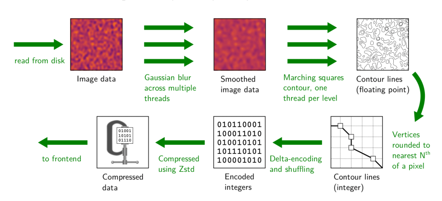
In the end, issue (1) was deemed to be too much of a drawback, as user rely on CARTA for accurate representations of their data. Instead, we opted for a hybrid contouring approach: Contours poly-lines are generated on the backend over a number of threads, before being compressed (covered in Part 2) and sent to the frontend. The frontend then decompresses the contours and renders them using WebGL (covered in Part 3). An outline of the contour generation pipeline is shown in Figure 1.

Figure 1: Outline of contour generation and compression on backend

Smoothing

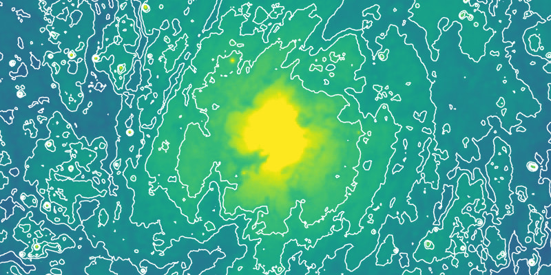
Astronomy images are often rather noisy, and contours generated raw images are often full of noise. An example of this is shown in Figure 2.

Figure 2: M51 contours with no smoothing

The contouring algorithm is approximately $O(W \times H \times L)$ , where $W$ and $H$ are the width and height of the image respectively, and $L$ is the number of contour levels to generate. In practise, performance depends heavily on the fraction of points near the contour levels. Poorly chosen contour levels near the noise threshold take a lot longer to generate, because there are so many points in the image at which pixels cross the level.

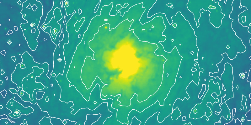
Smoothing the image prior to contouring results in a lowered noise level, and contours can be generated to highlight real sources, rather than noise. Two smoothing modes are commonly used in this step: Block-averaging (each $N^2$ block of pixels is replaced by a value represting the entire block, usually the mean) and Gaussian smoothing (the image is convoluted with a 2D Gaussian kernel of size $M^2$ ). Block-averaging reduces the size of the image to $W \times H / N^2$ , while Gaussian smoothing retains the image size. As such, contours generated from block-averaged images tend to lack detail, as shown in Figure 3.

Figure 3: M51 contours with block smoothing

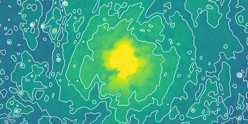
The reduction in image size means the contouring is now $O(W \times H \times L / N^2)$ , while contouring of Gaussian smoothed images remains $O(W \times H \times L)$ . In practice, both smoothing approaches also improve performance by lowering the noise level. Gaussian smoothing tends to produce much clearer contours, as shown in Figure 4.

Figure 4: M51 contours with Gaussian smoothing

DS9 defaults to block smoothing, as Gaussian smoothing can be computationally expensive if not carefully optimised. For CARTA, we wanted to make Gaussian smoothing the default smoothing, as we felt it would produce better contours, and we were confident that we could improve smoothing performance over DS9.

In order to do this, we chose to use a two-pass smoothing process, as Gaussian smoothing is separable, as long as the Gaussian kernel is symmetric. The image is first smoothed by a 1D kernel in the horizontal direction, and then smoothed in the vertical direction. This reduces the complexity per pixel from $O(M^2)$ to $O(M)$ . Normally, a two-pass smoothing process requires twice as much memory for the intermediary image, but we use a fixed buffer size of 200 MB and perform the smoothing on strips of the original image. Each strip is processed in parallel, with each thread smoothing a sub-strip. AVX vector instructions (with a fallback to SSE) allow each thread to process four pixels at once.

Figure 5: Gaussian blur speed in CARTA 1.3

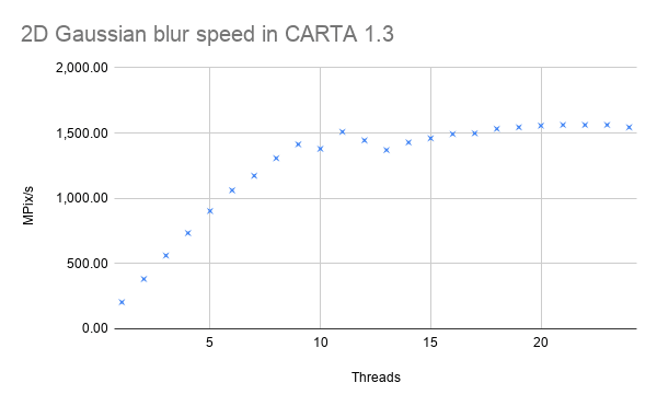
A 12-core AMD Ryzen 3900x was used for benchmarking, with a 400 megapixel image and a kernel width of 7 pixels. As shown in Figure 5, performance scales almost linearly with the number of threads, up to about 8 or 9 threads, after which, performance plateaus at about 1500 MPix/s, as the bottleneck shifts to memory bandwidth. A quad-channel processor such as the Ryzen 3960x would allow for near-linear scaling up to a much higher number of threads.

Comparing performance to that of DS9 with identical smoothing settings, CARTA 1.3's smoothing is up to 1000x faster 🚀🚀🚀

In the rest of this series, I'll discuss how the contour poly-lines are efficiently compressed and finally rendered in the browser.