TomTom Routing

While working with the Google Mobility Data I stumbled upon the TomTom Traffic Index. I then learned that TomTom has a public API which exposes a bunch of useful and interesting data.

Seemed like another opportunity to create a smaller R package. Enter {tomtom}.

{tomtom} Package

The {tomtom} package can be found here.

Install the package.

remotes::install_github("datawookie/tomtom")

Load the package.

library(tomtom)

API Key

Getting a key for the API is quick and painless. I stored mine in the environment then retrieved it with Sys.getenv().

TOMTOM_API_KEY = Sys.getenv("TOMTOM_API_KEY")

Then use set_api_key() to let {tomtom} know about the key.

set_api_key(TOMTOM_API_KEY)

Routing

So far I’ve only implemented a function for the routing endpoint. Let’s give that a try.

First set up a series of locations on a tour spanning South Africa.

locations <- tribble(
  ~label, ~lon, ~lat,
  "Durban", 31.05, -29.88,
  "Port Elizabeth", 25.6, -33.96,
  "Cape Town", 18.42, -33.93,
  "Johannesburg", 28.05, -26.20
)

Now convert these into an sf object.

library(sf)

locations <- st_as_sf(
  locations,
  coords = c("lon", "lat"),
  remove = FALSE, crs = 4326
)
locations

Simple feature collection with 4 features and 3 fields
Geometry type: POINT
Dimension: XY
Bounding box: xmin: 18.42 ymin: -33.96 xmax: 31.05 ymax: -26.2
Geodetic CRS: WGS 84
# A tibble: 4 x 4
  label lon lat geometry
* <chr> <dbl> <dbl> <POINT [°]>
1 Durban 31.0 -29.9 (31.05 -29.88)
2 Port Elizabeth 25.6 -34.0 (25.6 -33.96)
3 Cape Town 18.4 -33.9 (18.42 -33.93)
4 Johannesburg 28.0 -26.2 (28.05 -26.2)

And then call the calculate_route() function.

routes <- calculate_route(locations)

# A tibble: 3 x 6
  route leg distance time delay points                   
  <fct> <fct> <int> <int> <int> <list>                   
1 1 1 910426 37965 673 <tibble[,2] [11,125 × 2]>
2 1 2 750144 26928 0 <tibble[,2] [6,902 × 2]> 
3 1 3 1403495 46516 0 <tibble[,2] [7,365 × 2]> 

The results are broken down into legs (three legs between the four locations). The distance and time fields are in metres and seconds respectively.

Unnesting the points field we can plot out the suggested route.

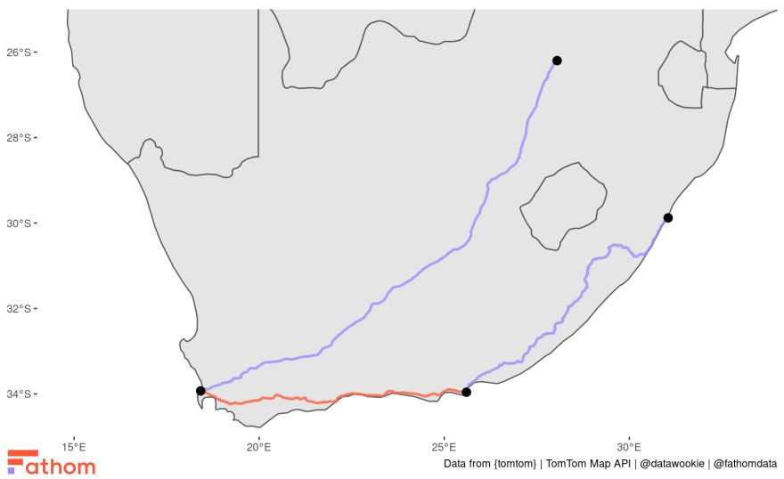
Makes sense! This is both a direct and scenic way to get from Durban to Cape Town via Port Elizabeth and then return to Johannesburg. The leg between Port Elizabeth and Cape Town is particularly lovely.

Taking the (not so) Scenic Route

Is that the only way to travel between those destinations? Hell no! There are lots of options. And we can access them via {tomtom} too.

Suppose we want to consider the best route along with a few alternatives.

routes <- calculate_route(locations, alternatives = 3)

# A tibble: 12 x 5
   route leg distance time delay
   <fct> <fct> <int> <int> <int>
 1 1 1 910426 37965 673
 2 1 2 750144 26928 0
 3 1 3 1403495 46517 0
 4 2 1 989397 39654 0
 5 2 2 780416 29647 0
 6 2 3 1437322 49943 0
 7 3 1 990812 43337 0
 8 3 2 839345 30480 0
 9 3 3 1591759 53469 0
10 4 1 941134 38585 83
11 4 2 867969 31817 0
12 4 3 1515709 51730 0

Now we have four routes, each of which has three legs. It’s easier to compare the routes if we summarise them.

# A tibble: 4 x 4
  route km hour avg_speed
  <fct> <dbl> <dbl> <dbl>
1 1 3064. 30.9 99.0
2 2 3207. 33.1 96.8
3 3 3422. 35.4 96.8
4 4 3325. 33.9 98.0

The avg_speed field is in units of km / hour. The first route is preferred because it’s faster and significantly shorter. The other options are not too bad though.

Let’s take a look at the distance and time for each of these routes broken down by leg.

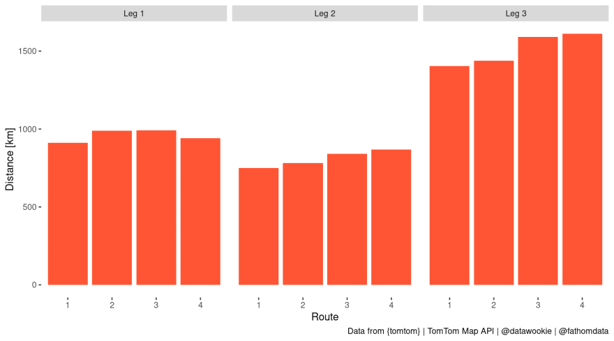
It’s apparent that the first route is both quicker and shorter across all three legs. Definitely the preferred way to get around the country if you want to save time and fuel.

Finally we’ll compare the actual routes.

Each route will present a very different view of the land. I particularly like the option which heads off into the Northern Cape on the leg from Cape Town to Johannesburg. That’s a seriously underappreciated part of the country.