Convolutional Sequence to Sequence

Recurrent neural networks (RNNs) with LSTM or GRU units are the most prevalent tools for NLP researchers, and provide state of the art results on many different NLP tasks, including language modeling (LM), neural machine translation (NMT), sentiment analysis, and so on. However, a major drawback of RNNs is that since each word in the input sequence are processed sequentially, they are slow to train.

Most recently, Convolutional Neural Networks - traditionally used in solving most of Computer Vision problem, have also found prevalence in tackling problems associated with NLP tasks like Sentence Classification, Text Classification, Sentiment Analysis, Text Summarization, Machine Translation and Answer Relations.
Back in 2017, a team of researchers from Facebook AI research released an interesting paper about Sequence to Sequence learning with Convolutional neural networks(CNNs), where they tried to apply CNNs to problems in Natural Language Processing.

In this post, I’ll try to summarize this paper on how CNN's are being used in machine translation.

What are Convolutional Neural Networks and their effectiveness for NLP?

Convolutional Neural Networks (CNNs) were originally designed to perform deep learning for computer vision tasks, and have proven highly effective. They use the concept of a “convolution”, a sliding window or “filter” that passes over the image, identifying important features and analyzing them one at a time, then reducing them down to their essential characteristics, and repeating the process.

Now, lets see how CNN process can be applied to NLP.

Neural networks can only learn to find patterns in numerical data and so, before we feed a text into a neural network as input, we have to convert each word into a numerical value. It starts with an input sentence broken up into words and transformed to word embeddings - low-dimensional representations generated by models like word2vec or GloVe or by using a custom embedding layer. The text is organized into a matrix, with each row representing a word embedding for the word. The CNN’s convolutional layer “scans” the text like it would an image, breaks it down into feature. 
The following image illustrates how the convolutional “filter” slides over a sentence, three words at a time. This is called a 1D convolution because the kernel is moving in only one dimension. It computes an element-wise product of the weights of each word, multiplied by the weights assigned to the convolutional filter. The resultant output will be a feature vector that contains about as many values as there were in input embeddings, so the input sequence size does matter.

A convolutional neural network will include many of these kernels (filters), and, as the network trains, these kernel weights are learned. Each kernel is designed to look at a word, and surrounding word(s) in a sequential window, and output a value that captures something about that phrase. In this way, the convolution operation can be viewed as window-based feature extraction.

We'll be building a machine learning model to go from once sequence to another, using PyTorch and TorchText. This will be done on German to English translations, but the models can be applied to any problem that involves going from one sequence to another, such as summarization, i.e. going from a sequence to a shorter sequence in the same language.
Before we delve deep into the code, lets first understand the model architecture as mentioned in the paper.
Lets recall our general RNN based encoder decoder model, 

We use our encoder (green) over the embedded source sequence (yellow) to create a context vector (red). We then use that context vector with the decoder (blue) and a linear layer (purple) to generate the target sentence.

How convolutional sequence to sequence model work?

An architecture proposed by authors for sequence to sequence modeling is entirely convolutional. Below diagram outlines the structure of convolutional sequence to sequence model.

Like any RNN based sequence to sequence structure CNN based model uses encoder decoder architecture, however here both encoder and decoder are composed of stacked convolutional layers with a special type of activation function called Gated Linear Units. In the middle there is a attention function. The encoder extracts features from the source sequence, while decoder learns to estimate the function that maps the encoders hidden state and its previous generated words to the next word. The attention tells the decoder which hidden states of the encoder to focus on.

 
A concept of positional embedding, is been introduced in this model. Well, what do we mean by positional embedding?
In CNN, we process all the words in a sequence simultaneously, it is impossible to capture the sequence order information like we do in RNNs (a timeseries based model). In order to use the sequence information of the sequence, the absolute position information of the tokens needs to be injected into the model and we need to explicity sent this information to the network.  This works just like a regular word embedding but instead of mapping words, it maps the absolute position of a word to a dense vector. The position embeding output will be added on the word embeding. With this additional information, the model knows which part of the context it is handling.

The paper also applies residual connection between the blocks in both the encoder and the decoder, which allows for deeper convolutional network. 

Why residual connection?
Models with many layers often rely on shortcut or residual connections. When we stack up convolutional layers to form a deeper model, it becomes harder and harder to optimize since the model has a lot of parameters, resulting in poor performance and also the gradient values start exploding and becomes very difficult to handle. This is solved by adding a residual block (skip connections) i.e to add the previous blocks output onto the current block directly. This technique makes the learning process easier and faster, enabling the model to go deeper, also helps improve the accuracy.

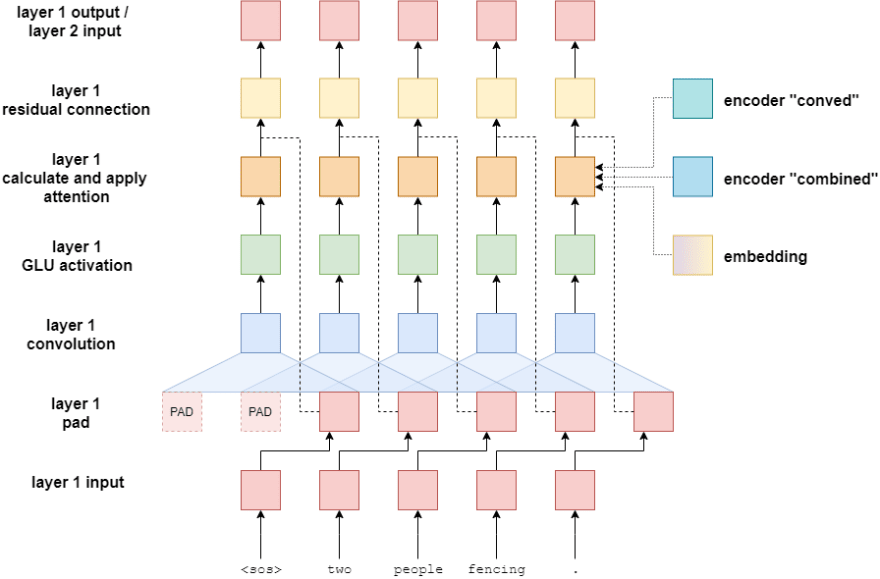
Encoder

Let's now have a closer look at the Encoder structure.

• We take the German sentence add padding at the start and end of the sentence and split those into tokens. This is because, the CNN layer is going to reduce the length of the sentence, to maintain same sentence length we add padding.
• We first send it to the embeding layer to get the word embedding, we also need to encode the position of the word, so we will be literally sending the position(index postion of the words) to another similar embeding layer to get the positional embeddings.
• We then do a element wise sum of word embedding and postional embedding, that is going to result in a combined embedding which is a element wise vector (This layer knowns the word and also has encoded even the location of the word) .
• This vector goes into a Fully connected layer because we need to convert it into a particular dimention and also, to help increase capacity and extract information, basically to convert these simple numbers into something which is more complex (like rearranging of features).
• The ouput of each of these FC layer is simultaneously sent to the multiple convolution blocks.
• For each of the information that is going into the convolutional block, we are going to get individual outputs.
• This output is again sent to another fully connected layer, because the output of the convolution need to be converted into the embedding dimension of the encoder.
• The final vector will have the embedding equal to the number of dimension we want.
• We also add a skip connection the output of the final FC layer gets added with the element wise sum of word and position embeding , i.e we are sending the whole word along with the position of the word to the decoder as convolutional layer might loose the positional information.

Finally, from the encoder block we will be sending two outputs to the decoder, one is the conved output and another is combined vector (which is combination of transformed vector and embedding vector)
i.e suppose we have 6 tokens, we will be getting 12 context vectors, 2 context vectors per token, one from conved and another from combined.

Convolutional Blocks

Lets now see the convolutional block within encoder architecture

• As mentioned earlier we pass the padded input sentence to the CNN block, this is because the CNN layer is going to reduce the length of the sentence, and we need to ensure that the length of the input sentence getting into the convolution block is equal to the length of the sentence going out of the convolution block.
• We will be then convolving the padded output using a kernel size of 3 (odd size)

• The output of this is sent to a special kind of acivation GLU (Gated Linear Unit) activation.

  How GLU activation works?

  The output of convolutional layer i.e input to GLU is split into two halves A and B, half the input (A) would go to sigmoid and we would then do a element wise sum of both. Sigmoid acts as a gate, determining which part of B are relevant to the current context. The larger the values of entry in A the more important that corresponding entry in B is. The gating mechanisn of the models enables to select the effective parts of the input features in preducting the next words. Since the GLU is going to reduce the input to half, we would be doubling the input to the convolution block.

  

• Then we add a residual connection i.e The output of the combined vector is going to be added as a skip connection to the output of the GLU, this done just to avoid any issues associated with the convolutional layers, this skip connections ensures smooth flow of gradients

This concludes a single convolutional block. Subsequent blocks take the output of the previous block and perform the same steps. Each block has their own parameters, they are not shared between blocks. The output of the last block goes back to the main encoder - where it is fed through a linear layer to get the conved output and then elementwise summed with the embedding of the token to get the combined output.

Decoder

The Decoder is very similar to Encoder, but with few changes.

• We will passing the whole output for the prediction, like encoder we will first pass the tokens to the embeding layer to get the word and postional embedding.
• Add both the word and postional embedding using element wise sum, pass it to the fully connected layer, which then goes to the convolutional layer.
• The convolutional layer accepts two additional inputs i.e the encoder conved and encoder combined (this is to feed encoder information into the decoder), we also pass the embedding vector as a residual connection to the convolution layer. Unlike the encoder, the resnet connection or skip connection goes only to the convolution block it doesnot go to the output of the convolution block because we have to use the information to predict the output.
• This goes to two layer linear network (FC layer) to make the final prediction.

Decoder Conv Blocks

Let's now see the decoder convolutional blocks, this is similar to the one within encoder. However there are few changes.

For encoder the input sequence is padded so that the input and output lengths are the same and we would pad the target sentence in the decoder aswell for the same reason. However, for decoder we only pad at the beginning of the sentence, the padding makes sure the target of the decoder is shifted by one word from its input. Since we are processing all the target sequence simultaneously, so we need a method of not only allowing the filter to translate the token that we have to the next stage, but we also need to make sure that the model will not learn to output the next word in the sequence by directly copying the next word, without actually learning how to translate.

If we don't pad it at the beginning (as shown below), then the model will see the next word while convolving and would literally be copying that to the output, without learning to translate

Attention

The model also adds a attention in every decoder layer and demonstrate that each attention layer only adds a negligible amount of overhead.The model uses both encoder conved and encoder combined, to figure out where exactly the encoder want the model to focus on while making the prediction

• Firstly, we take the conved output of a word from the decoder, do a element wise sum with the decoder input embedding to generate combined embedding
• Next, we calculate the attention between the above generated combined embedding and the encoder conved, to find how much it matches with the encoded conved
• Then, this is used to calculate the weighted sum over the encoded combined to apply the attention.
• This is then projected back up to the hidden dimenson size and a residual connection to the initial input is applied to the attention layer.

This can be seen as attention with multiple ’hops’ compared to single step attention

Seq2Seq

For the final part of the implementation, we'll implement the seq2seq model. This will stitch the Encoder and Decoder together:

• Firstly token is sliced off from the target sentence as we do not input this token to the decoder.
• The encoder receives the input/source sentence and produces two context vectors for each word:
  • encoder_conved (output from final encoder conv. block) and
  • encoder_combined [encoder_conved plus (elementwise) src embedding plus positional embeddings]
• The decoder takes in all the target sentence at one to produce the prediction of output/target sentence

Inference

Following are the steps that we taken during inference:

• Firstly, ensure our model is in evaluation mode, which it should "always" be for inference
• When a new unseen sentence is passed, we first convert that to lower case and tokenize the sentence
• append the <sos> and <eos> tokens
• map the tokens to their indexes i.e corresponding integer representation fron vocab
• convert it to a tensor and use unsqueeze operation to add a batch dimension
• feed the source sentence into the encoder using torch.no_grad() block to ensure no gradients are calculated within the block to reduce memory consumption and speed things up.
• create a list to hold the output sentence, initialized with an <sos> token
• while we have not hit a maximum length
  • convert the current output sentence prediction into a tensor with a batch dimension
  • place the current output and the two encoder outputs into the decoder
  • get next output token prediction from decoder
  • add prediction to current output sentence prediction
  • break if the prediction was an token
• convert the output sentence from indexes to tokens
• return the output sentence (with the token removed) and the attention from the last layer

Conclusion

Compared to RNN models convolution models have two advantages.

• First, it runs faster because convolution can be performed in parallel. By contrast, RNN needs to wait for the value of the previous timesteps to be computed.
• Second, it captures dependencies of different lengths between the words easily. In a group of stacked CNN layers, the bottom layers captures closer dependencies while the top layers extract longer (complex) dependencies between words.

Having said that when comparing RNN vs CNN, both are commonplace in the field of Deep Learning. Each architecture has advantages and disadvantages that are dependent upon the type of data that is being modeled.

From the abstract of the paper, the authors claim to outperform the accuracy of deep LSTMs in WMT’14 English-German and WMT’14 English-French translation at an order of magnitude faster speed, both on GPU and CPU.

Pytorch implementation to this can be found here