Optimising linear regression: A guide to applying gradient descent

Linear regression is a statistical technique that helps us understand and predict relationships between variables. It is widely used in data science and machine learning.

At its core, linear regression involves finding the best-fitting line through a set of data points, allowing us to make predictions about future values based on past observations.

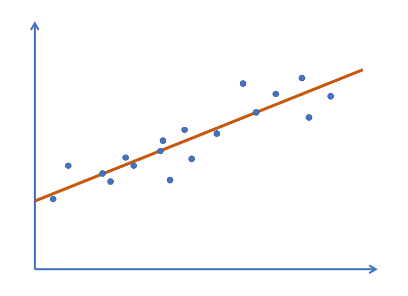
Finding the line can be a complex and computationally-intensive task, especially when dealing with large datasets.

Enter gradient descent... an optimisation algorithm that we can use to find the best-fitting line by iteratively adjusting its parameters.

It's worth noting that linear regression is a form of supervised learning where our algorithm is trained on "labelled" data. This simply reflects the fact that, within the available data, the inputs have corresponding outputs or labels.

In this blog, we will look at the maths, specifically the partial derivatives, involved in applying gradient descent to linear regression.

Model

Given a training set, our aim is to model the relationship so that our hypothesis $\hat{y}$ is a good predicator for the corresponding value of $y$ .

For simple or univariate linear regression, our model can be expressed as:

$$\hat{y} = \theta_0 + \theta_1{x_1}$$

And for multivariate linear regression:

$$\hat{y} = \theta_0 + \theta_1{x_1} + \theta_2{x_2} + ... + \theta_j{x_j}$$

Loss function

We can measure the accuracy of our hypothesis $\hat{y}$ by calculating the mean squared error - including a $\frac{1}{2}$ to simplify the derivatives that follow later.

$${Loss, l} = \frac{1}{2m}\sum_{i=1}^{m}(\hat{y} - y)^2$$

Gradient descent

We need to minimise the loss to ensure that $\hat{y}$ is a good predicator of $y$ .

Gradient descent is well described elsewhere but the principle is that we adjust the $\theta$ parameters until the loss is at the very bottom of the curve.

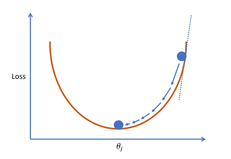
The adjustment is achieved by repeatedly taking the derivative of the loss function (the tangent line) to infer a movement to the right (gradient is negative) or the left (gradient is positive).

The size of each step is relative to a fixed hyper parameter $\alpha$ which is called the learning rate. Typical values for $\alpha$ are 0.1, 0.01 and 0.001.

This approach can be articulated as:

$$\theta_j = \theta_j - \alpha\dfrac{\mathrm{d}l}{\mathrm{d}\theta_j}$$

There are three types of gradient descent:

1. Batch gradient descent: Update the $\theta$ parameters using the entire training set; slow but guaranteed to converge to the global minimum
2. Stochastic gradient descent: Update the $\theta$ parameters using each training example; faster but may not converge to the global minimum due to randomness
3. Mini batch gradient descent: Update the $\theta$ parameters using a small batch of training examples; compromise between efficiency and convergence

Gradient descent derivatives

Imagine we have the following training data:

x1	x2	y
5	6	31.7
10	12	63.2
15	18	94.7
20	24	126.2
...	...	...
...	...	...
35	42	220.7

Our model will be:

$$\hat{y} = \theta_0 + \theta_1{x_1} + \theta_2{x_2}$$

Let's say we want to apply stochastic gradient descent.

Here are the steps we need to follow:

1. Set $\alpha$ to 0.001 (say) and $\theta_0$ , $\theta_1$ and $\theta_2$ to random values between -1 and 1
2. Take the first training example and use gradient descent to update $\theta_0$ , $\theta_1$ and $\theta_2$
3. Repeat step 2 for each of the remaining training examples
4. Repeat the process from step 2 another 1000 times

Let's look at the expressions and derivatives needed, starting with the loss.

When we consider just one training example at a time, as with stochastic gradient descent, $m = 1$ .

As such, the loss between our hypothesis $\hat{y}$ and $y$ can be described as:

$${Loss, l} = \frac{1}{2}(\hat{y} - y)^2$$

Our gradient descent equation is:

$$\theta_j = \theta_j - \alpha\dfrac{\mathrm{d}l}{\mathrm{d}\theta_j}$$

To apply it, we need to determine:

$$\dfrac{\mathrm{d}l}{\mathrm{d}\theta_j}$$

Using the chain rule, we can say that:

$$\dfrac{\mathrm{d}l}{\mathrm{d}\theta_j} = \dfrac{\mathrm{d}l}{\mathrm{d}(\hat{y} - y)} . \dfrac{\mathrm{d}(\hat{y} - y)}{\mathrm{d}\theta_j}$$

One of the linearity rules of derivatives tells us that when differentiating the addition or subtraction of two functions, we can differentiate the functions individually and then add or subtract them.

This means we can say:

$$\dfrac{\mathrm{d}l}{\mathrm{d}\theta_j} = \dfrac{\mathrm{d}l}{\mathrm{d}(\hat{y} - y)} . \left[ \dfrac{\mathrm{d}\hat{y}}{\mathrm{d}\theta_j}- \dfrac{\mathrm{d}y}{\mathrm{d}\theta_j} \right]$$

Since $y$ does not change with respect to $\theta$ :

$$\dfrac{\mathrm{d}y}{\mathrm{d}\theta_j} = 0$$

Therefore:

$$\dfrac{\mathrm{d}l}{\mathrm{d}\theta_j} = \dfrac{\mathrm{d}l}{\mathrm{d}(\hat{y} - y)} . \dfrac{\mathrm{d}\hat{y}}{\mathrm{d}\theta_j}$$

Let's now consider the two parts to this derivative, starting with the first:

$$\dfrac{\mathrm{d}l}{\mathrm{d}(\hat{y} - y)}$$

We can reduce this down:

$$\dfrac{\mathrm{d}l}{\mathrm{d}(\hat{y} - y)} = 2.\frac{1}{2}(\hat{y} - y) = (\hat{y} - y)$$

Now let's consider the second part of the derivative:

$$\dfrac{\mathrm{d}\hat{y}}{\mathrm{d}\theta_j}$$

We can this simplify this for $\theta_0$ , $\theta_1$ and $\theta_2$ as follows:

$$\dfrac{\mathrm{d}\hat{y}}{\mathrm{d}\theta_0} = \dfrac{\mathrm{d}(\theta_0 + \theta_1{x_1} + \theta_2{x_2})}{\mathrm{d}\theta_0} = 1$$

$$\dfrac{\mathrm{d}\hat{y}}{\mathrm{d}\theta_1} = \dfrac{\mathrm{d}(\theta_0 + \theta_1{x_1} + \theta_2{x_2})}{\mathrm{d}\theta_1} = x_1$$

$$\dfrac{\mathrm{d}\hat{y}}{\mathrm{d}\theta_2} = \dfrac{\mathrm{d}(\theta_0 + \theta_1{x_1} + \theta_2{x_2})}{\mathrm{d}\theta_2} = x_2$$

Let's now combine what we've worked out.

We found that:

$$\theta_j = \theta_j - \alpha\dfrac{\mathrm{d}l}{\mathrm{d}\theta_j}$$

Where:

$$\dfrac{\mathrm{d}l}{\mathrm{d}\theta_j} = \dfrac{\mathrm{d}l}{\mathrm{d}(\hat{y} - y)} . \dfrac{\mathrm{d}\hat{y}}{\mathrm{d}\theta_j}$$

And:

$$\dfrac{\mathrm{d}l}{\mathrm{d}(\hat{y} - y)} = (\hat{y} - y)$$

Therefore we can say:

$$\theta_0 = \theta_0 - \alpha\dfrac{\mathrm{d}l}{\mathrm{d}\theta_0} = \theta_0 - \alpha(\hat{y} - y)$$

$$\theta_1 = \theta_1 - \alpha\dfrac{\mathrm{d}l}{\mathrm{d}\theta_1} = \theta_1 - \alpha(\hat{y} - y)x_1$$

$$\theta_2 = \theta_2 - \alpha\dfrac{\mathrm{d}l}{\mathrm{d}\theta_2} = \theta_2 - \alpha(\hat{y} - y)x_2$$

We now have all of the expressions needed to apply gradient descent. Over 1000 iterations, we might expect to see the total loss per iteration decrease like this.

In this post, we looked at the maths, specifically the partial derivatives, involved in applying gradient descent to linear regression.

For more information, check out Andrew Ng's Stanford CS229 lecture on Linear Regression and Gradient Descent.