In most situations, the lookup value is a unique known identifier, so we can use the exact match to return the exact corresponding information in the same row. Sometimes, the lookup value is unknown, in this situation we can use an approximate match is used to find the closest or nearest match based on given the criteria. Here is the tutorial to find the approximate match with the VLOOKUP function in Excel Search Box. Let’s get into this article!! Get an official version of ** MS Excel** from the following link: https://www.microsoft.com/en-in/microsoft-365/excel
Steps to find an approximate match:
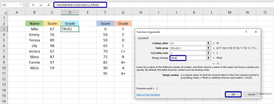
Refer to the below image to know how to find an approximate match in Excel by using the search box.
- For instance, In the data table below we need to find the grades of the students based on their scores.

- We select the cell where the result to be displayed.
- Click the “Formula” tab from the Ribbon.

- Here, we will select the “Insert Function” option.

- Search for “VLOOKUP” then select to “Go” option.

- The VLOOKUP function will appear in the below box and click on the “OK” button.

- Now, it will open the “Function Arguments” window. In the 1st box , you need to enter the lookup value which you want to be found.

- In the 2nd box, we will select the data range from the worksheet.

- The next box consists of the column number , where the lookup value will available.

- In the last box, type “TRUE” to search the approximate matching value** [FALSE = Exact match], and click the “Ok”** button.
- The result will display in the selected cell.
- Finally, drag-down the result cell, it will display the results in all cells with a matching value.

Verdict:
That’s all. This is how we find the approximate match from the table by using the VLOOKUP function in the Excel Search box. Leave a comment or reply below – let me know what you think! To learn more about Excel, check out Geek Excel!!

Top comments (0)