The most difficult part of week 2 is taking the formulas and converting them into Octave. Especially, if you don't quite grasp the formula notations and Octave is new.
I will walk through some of the boiler plate code regarding Gradient Descent, the hypothesis function, cost function, and try to develop some intuition to move things forward. I will also point out my own gaps of understanding in the hopes that I can fill them in later.
Know Your Resources
As I was writing these notes I stumbled on the "Resources" section which has been immensely helpful and clarified quite a lot. I highly recommend reading the lecture notes for each week as they clarify the videos and other resources quite a lot.
The Shape of Matrices
The shapes of two matrices dictate whether or not you can compute the dot product of the two.
In Dr. Ng's slides on Vectorization he calculates the following hypothesis function using an iterative notation (summation) and a vectorized notation (transpose and dot product):

Note that in this case "x_j" (x subscript j) indicates the value of feature "j". The Week 2 Lecture Notes under resources is incredibly helpful here. "x" is a column vector of feature values. Perhaps its the square footage of each house in the data set or the number of floors for each house. Whereas the thetas represent "weights" for each feature such as the price per floor or price per square foot.
The week 2 notes expand this function like so:
hθ(x)=θ_0+θ_1x_1+θ_2x_2+θ_3x_3+⋯+θ_nx_n
This hypothesis function takes a row or instance from the data set, say a house, and takes each of its features x_y multiplied against their corresponding θ_y or weight. The value for theta is what we attempt to discover through Gradient Descent.
A part of the exercise I don't quite understand is that a column of ones is added to X. This column of ones will be paired with θ_0 when calculating the hθ(x) function. This is definitely a part I have confusion on.
Getting back to vectorization. Seeing that the summation form of the hypothesis function can be represented as hθ(x)=θ_0+θ_1x_1+θ_2x_2+θ_3x_3+⋯+θ_nx_n makes it a lot easier to connect this to matrix multiplication where you multiply each value of a row times each value of a column in two matrices and sum them to get a new value.
Since we know x and theta are column vectors lets see how the vectorized version of the hypothesis function would actually work.
% initialize column vector a. ; starts a new row.
octave:8> a = [ 1; 2; 3; 4; 5; 6 ]
a =

   1
   2
   3
   4
   5
   6

% initialize column vector b. ; starts a new row.
octave:9> b = [ 1; 2; 3; 4; 5; 6]
b =

   1
   2
   3
   4
   5
   6

% and voila a transpose dot product b returns a single value.
octave:10> a' * b
ans =  91
Continuing on the Programming Tips from Mentors has a really helpful clarification to reach a fully vectorized solution:
"h(x) = theta' * x" vs. "h(x) = X * theta?"
Lower-case x typically indicates a single training example.
Therefore X potentially has multiple "x" or single training examples. A training example in our case would be a row and each column in the row a feature for that training sample.
Remember the Σ(h(x_j) - y)? The sigma tells us we need to calculate this for all rows of X. Since X has a column for each row of theta we can multiply them together as we did theta' * x.
Calculating Cost
The programming exercise has this definition for the cost function:
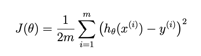
The cost function J(θ) has a very minor detail where it plugs x^(i) into the hypothesis function. Meaning for a particular feature/column calculate the hypothesis over all training examples. The summation symbols to the left indicate that this should be done for each column in the data set. You could do this iteratively, but its a lot easier when you realize X * theta means the same thing. X * theta means multiply every training example (row) times every theta (column) aka θ_0 + θ_1x_1.
Instead of subtracting one x from one y we can now use the h(x) vector calculated above subtract the y matrix.
The interesting bit though is that originally y was a single column and so was X:
X = data(:, 1); y = data(:, 2);
disp(size(X))
disp(size(y))

% 97 1
% 97 1
However, X is reassigned to have two columns. Subtraction between these two matrices should not be possible, but Octave allows it via "broadcasting".
Since y has fewer dimensions Octave transforms it into a matrix consisting of [y, y] to match X dimension of 97 x 2. At this point the ones column on X is a throw away column used to provide proper shape. X[:,2] and y[:] have a relation recorded in the original dataset, but the arbitrary ones column should have no such relation. Perhaps their hint about dimensional analysis makes this make sense.
The next trick comes when trying to figure out how to take h(x) - y to the power of 2. Remember everything in the function definition is defined iteratively so what the function is telling us is to square each element of the matrix, not the entire matrix.
Your intuition might be to use Octave's broadcast exponentiation (x.^y or x.**y) provides this for us:
Element-by-element power operator. If both operands are matrices, the number of rows and columns must both agree, or they must be broadcastable to the same shape. If several complex results are possible, the one with smallest non-negative argument (angle) is taken. This rule may return a complex root even when a real root is also possible. Use realpow, realsqrt, cbrt, or nthroot if a real result is preferred.
Which I think actually works since its an element-by-element power operation, but the vectorized version is described in the week 2 lecture notes as follows:

This preserves the iterative squaring of each term by multiplying each position in the matrix by itself. Pretty neat!
Conclusion
There is so much more I still don't quite understand, but at this point I have a framework for converting iterative solutions to vectorized solutions. Some of intuition behind the hypothesis function and the cost functions themselves are still beyond me. Why is understanding "dimensional analysis" important? Why is it OK to do broadcast subtraction of (X * theta) - y?

Latest comments (0)