In the previous article we outlined the various classifications of Data Structures that exist and some of the various Algorithms that are mainly performed on Data Structures. In this article we shall build upon those concepts by delving into the following: Arrays, Linked Lists, Trees, and Searching.
1. Arrays
This could be referred to as an indexed collection of data. Generally, arrays are declared with an opening square bracket and ended with a closing square bracket. A comma is put between each element and the data types enclosed within an array should all be of the same type, like this:
//examples of arrays
const sandwich = ["peanut butter", "jelly", "bread"];
//or
int  scores[3] = [77, 73, 81];
When accessing the array, we use zero-based indexing such that to access the third element (81) in the scores array we could say:
scores[2];
The disadvantage of using arrays is that it requires an allocation of a fixed size, back-to-back in memory. This makes it difficult to add new elements to the array as there may be values stored in the memory addresses immediately after the address of the array.
One solution might be to allocate more memory where there’s enough space, and move our array there. This means we’ll need to allocate more memory to copy each of the original elements first, then add our new element and free the old array once we finish copying. Another solution may be to use a Linked List.
2. Linked Lists
When we have a large enough array, there might not be enough free memory contiguously, in a row, to store all of our values. Rather than allocate a fixed size of memory back-to-back, linked lists allow us to add elements in different parts of memory while adding references to those elements that point to the next node so as to stitch all the elements together. This combination of a data element with the reference pointer forms a node.

As demonstrated in the image above, when we want to insert a new value, we allocate enough memory for both the value we want to store, and the address of the next value. For the last value in the Linked List, we use the null pointer since there’s no next group.
With a linked list, we have the tradeoff of needing to allocate more memory for each value and pointer, in order to spend less time adding values.
3. Trees
Unlike arrays and linked lists that are linear data structures, trees outline a hierarchical relationship between data elements. A tree is another data structure where there are nodes; however, the nodes have two pointers and each node points to other nodes. This can be illustrated as shown in the figure below:
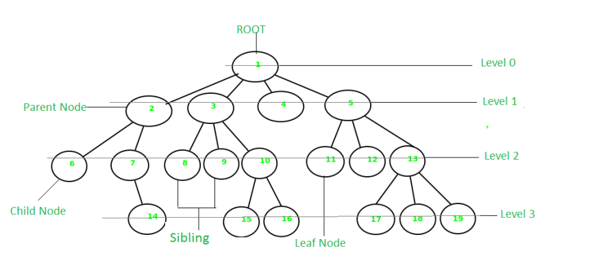
We might have a tree where the root node points to one node on the left and one node on the right. The nodes to the right and left of the root are Parent nodes and form the first hierarchical level of the tree. The immediate lower level nodes of the parent node are the children. Two children sharing a parent node are referred to as siblings. A node without a child is referred to as a leaf.
4. Searching
Since computers cannot look at all data elements at once, for arrays that are zero-indexed we can access the elements of an array of n items by going through index 0 to the highest index (which would be n-1). If the particular value of the element required matches the value that has been accessed, then we have achieved Searching.
There are algorithms for searching with varying levels of efficiency depending on their running times. To describe the running time of a program we use Big Ω notation, which describes the lower bound of number of steps for our algorithm (i.e. how few steps it might take in the best case). We also use Big O notation, which is the upper bound of number of steps for our algorithm (i.e. how many steps it might take in the worst case)
Some common running times:
O(n^2)
O(nlog n)
O(n)
O(log n)
O(1)
Ω(n^2)
Ω(nlog n)
Ω(n)
Ω(log n)
Ω(1)
An algorithm with running time of O(1) means that a constant number of steps is required, no matter how big the problem is. This is illustrated in the figure below:

In a linear data structure such as an array or linked list, if we didn’t know anything about the values, the simplest search algorithm would be going from left to right. This type of algorithm is referred to as Linear Search and it is not very efficient with a running time of O(n).
In a non-linear data structure such as a tree, to search for a number, we’ll start at the root node, and be able to recursively search the left or right subtree. Since we might have to keep dividing the number of elements by two until there are no more elements left, this type of algorithm is referred to as Binary Search and it has an upper bound of O(log n) . If the number we’re looking for is in the middle (i.e. where we happen to start) then the lower bound for binary search would be Ω(1).
Even though binary search might be much faster than linear search, it requires our elements to be sorted first. With a balanced binary search tree, the running time will be O(log n); however if our tree isn’t balanced, it can devolve into a linked list with running time of O(n).

Top comments (0)