Game of Life, the DTerminal edition

Yet another offshoot from my Advent of Code 2019 adventures (first half, second half, all solutions): on day 24, the challenge was to program a variant of Conway’s game of life, and I figured I might as well try my approach on the real thing!

A quick google for existing implementations yields three main approaches: nested for, shifting of matrix rows and columns, and repeated filtering of a coordinate data.frame. Visualisations tend to rely on R’s plotting capabilities, and more recently {gganimate}.

I used data.table for the computations, because it’s fast and succinct. Here’s the setup of the Game of Life universe, randomly seeding half of the cells as alive, and defining the relevant relative ‘neighbourhood’ of each cell through a small auxiliary table. For those unfamiliar with data.table, CJ() performs a cross-join to obtain all combinations of the vector arguments.

library(data.table)

dims <- c(49, 49)
universe <- CJ(x = seq(dims[1]), y = seq(dims[2]), k = 1, cell = FALSE)
universe[, cell := sample(c(FALSE, TRUE), prod(dims), TRUE)]

neighbours <- CJ(xd = -1:1, yd = -1:1, k = 1)[xd != 0 | yd != 0]

Next, we want to define a function to perform one step (or tick ) of the game. The basic approach is to do a full Cartesian join of the neighbourhood and the universe, to determine the neighbouring coordinates of each cell. We clip off at the edges (unlike a proper GoL universe, which is infinite), and aggregate grouped by the original cell coordinate to count the number of neighbours. data.table allows us to express all of this in a really compact manner:

gol_tick <- function(xy, sz, nb) {

  nb[xy, on = .(k), allow.cartesian = TRUE
    ][, nbx := x + xd][, nby := y + yd
    ][nbx >= 1 & nbx <= sz[1] & nby >= 1 & nby <= sz[2]
    ][xy, on = .(nbx = x, nby = y)
    ][, .(nnb = sum(i.cell)), by = .(x, y, cell, k)
    ][!cell & nnb == 3, cell := TRUE
    ][cell & (nnb < 2 | nnb > 3), cell := FALSE
    ][, nnb := NULL]

}

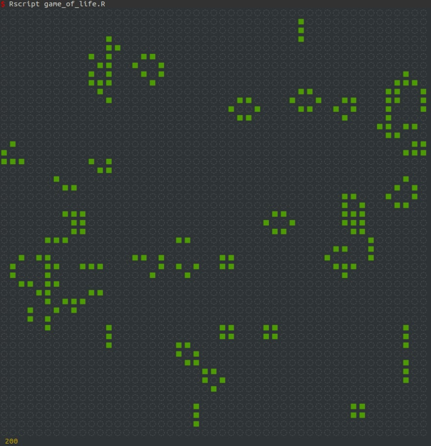
So how about some visuals - and perhaps a bit of interaction? I chose to do this in the terminal, just to make the point that you can easily create these old-school games fully in R! You will need an ANSI-capable terminal emulator though, such as the default Ubuntu one. Do make it large enough (or the font small enough).

First, the interaction part. To collect keypresses without pausing the universe to prompt the user, we need the {keypress} package. Usage is as simple as calling keypress(FALSE) to get the currently pressed key. Second, the visuals. Geometric unicode characters can provide a nice grid layout, but how do we ensure that we update the visuals with each tick, instead of spitting out an endless sequence of universe states into the terminal? The answer is ANSI escape codes, which allow you to colour the output, clear terminal lines, and crucially move the cursor back to a previous position. All of this is achieved simply by outputting strings starting with \033[ (or \u001B[), followed by the ANSI instruction. For a more user-friendly interface to many of these functionalities have a look at the {cli} package - but here is the fully manual approach:

library(keypress)

cat("\033[?25l")

repeat ({

  kp <- keypress(FALSE)

  universe[order(y, x)
    ][, cat(fifelse(.SD$cell, "\033[32;40m◼", "\033[90;40m◌"),
            "\033[K\n"),
      by = y]

  cat("\033[2K\033[33;40m", sum(universe$cell), "\n")

  if (kp == "q") break

  if (kp == "x") {
    new_cells <- sample(c(FALSE, TRUE), prod(dims), TRUE, c(9, 1))
    universe[, cell := cell | new_cells]
  }

  Sys.sleep(0.2)

  cat(paste0("\033[", dims[2] + 1, "A"))

  universe <- gol_tick(universe, dims, neighbours)

})

cat("\033[?25h")

The game speed is throttled using Sys.sleep(), and the number of cells currently alive are displayed at the bottom. Two keys will be interpreted: q exits the game, and x insert new cells at random locations, to bring some new life to the eventually oscillatory universe!

The full code can be found in this gist. Run Rscript game_of_life.R and you should be seeing something like this:

Now go forth and multiply!