Efficient Data Preprocessing for Machine Learning models.

Efficient Data Preprocessing.

Most of the raw datasets are incapable of producing any sort of pattern recognition. Machine Learning models will be quite inefficient on these datasets.
The quality of your Machine Learning algorithm depends on the quality of the dataset. Even the most advanced algorithms won’t function properly on bad data. Data needs to additionally go through a few steps before it can be used.

In this article, I will endeavor to simplify the exercise of data preprocessing.
This is what the process developers conventionally follow before the data is ready to be utilized by machine learning models.

Step 1: Importing the Machine Learning Libraries

A large number of things in programming do not require to be indited explicitly every time they are required. There are functions for them, which can simply be invoked.

import numpy as np

import matplotlib.pyplot as plt

import pandas as pd

Here, we have used the “as” keyword so as to refer to that library/modules using the given name. (Alias)

Step 2: Importing the Dataset

dataset = pd.read_csv("Data.csv")

Here, using a pandas method (read_csv), we were able to import the CSV file.

Note that in Machine Learning lingo, X refers to feature matrix and y refers to label matrix (output)

In the following lines, we have assigned a portion of the dataset to feature and label matrices.

X = dataset.iloc[:, :-1].values

y = dataset.iloc[:, -1].values

We have used the iloc method onto the dataframe to extract the values.
The iloc method can be used in this way :

df.iloc[, ].

**Note: **The : in Python selects all entries and :-1 in Python selects all entries except the last.
So, for example in X, we have assigned all the rows and all the columns except the last in the dataset.

The .values method returns a Numpy representation of the DataFrame.

Step 3: Looking out for missing Data

There is no guarantee that the dataset that you possess is clean. A lot of the raw datasets have missing values inside of them which are detrimental to the Machine Learning model.
You can choose to delete the entire row of the missing entry in the dataset but that can also potentially remove any sort of useful data entries.
There are several ways to handle this problem.
Here are 2 :

• Taking the mean of all the values in the column and replacing the missing data with the mean.

• Taking the median of all the values in the column and replacing the missing data with the median.

Commonly, mean is used for replacing missing data.
But, if in the dataset, a major outlier is present, the mean would render useless as the value of the outlier can potentially distort the mean and thus, the median is preferred.

We can use SimpleImputer class from sklearn.impute to do this task easily.

from sklearn.impute import SimpleImputer


# Creating an object from SimpleImputer class.

imputer = SimpleImputer(missing_values=np.nan, strategy="mean")

The SimpleImputer can take a few parameters :

1. missing_values : All of the specified occurrences will be imputed.

2. strategy : The imputation strategy. If set to mean, then it replaces missing values using the mean along each column. (Can only be used with numeric data)

We now have to train the data. It is called as fit. After training the data, we would now have to replace the missing values with the mean by using transform.

imputer.fit(X[:, 1:3])
X[:, 1:3] = imputer.transform(X[:, 1:3])

We can also do the above 2 lines in a single line like :

X[:, 1:3] = imputer.fit_transform(X[:, 1:3])

Step 4: Encoding Categorical data

In the dataset, we might encounter entries that are not numbers like texts. Although we can figure the context of the text, the algorithms, unfortunately, can’t as they rely solely on numbers. To overcome this problem, we “encode” the data.

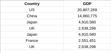In the first column, all the entries are in the form of text. This is an example of categorical data.

So, how to convert Categorical data to numerical data? There are 2 ways :

1. Integer Encoding: Each unique category is assigned an integer value.
2. One-Hot Encoding: Each unique category is assigned to a new column and only contain 0 or 1 corresponding to the column it has been placed.

Example For One-hot Encoding, Credits to @dan_s_becker on Twitter.

Encoding the Features (Independent Variable)

If we use Integer Encoding for categorical data, values like 0, 1, 2, and so on are encoded to these text entries. This certainly is understandable by the algorithms but, there's a catch. Say, if the US is assigned number 0, china to 1, Japan to 2 then aren’t we indirectly saying that Japan is greater than China or the US? But clearly, that’s not the intention here. So, this is not applicable here.

Instead, we have to use One-Hot encoding.

We can import them as well. We will have to use 2 classes.

from sklearn.compose import ColumnTransformer

from sklearn.preprocessing import OneHotEncoder

The first step is to create an object of the ColumnTransformerclass.

ct = ColumnTransformer(transformers=[("encoder", OneHotEncoder(), [0])] , remainder="passthrough")

In the first argument, we have to specify 3 things :

1. The kind of transformation. (Here, it is encoding and thus, we use encoder)

2. The kind of encoding we want to perform ( Here, we want One Hot encoding )

3. The indexes of the column we want to encode (Here, the first column this, we have mentioned 0 as in Python, indexes start from 0)

The second argument called remainder will be used to specify which columns to keep that won’t be applied. passthrough will make sure to keep all the columns that won’t be One-Hot encoded.

Now, we have to fit **and transform.**

X = ct.fit_transform(X)

Here’s a problem. The ct.fit_transform(X)does not return a NumPy array and we must have it as a NumPy array as Machine Learning models expect a matrix of NumPy array.

X = np.array(ct.fit_transform(X))

Encoding the labels (Dependent Variable)

If the labels contain binary values like “yes”, “no”, go for Integer Encoding.
It will convert these strings into 1 or 0.

For this, we have to import another class.

from sklearn.preprocessing import LabelEncoder

We now have to create an object of this class and after creating it, we can apply the fit_transform method.

le = LabelEncoder()

y = le.fit_transform(y)

We don’t have to convert it into a NumPy array as y is a dependent variable vector and there is no compulsion for it to be a NumPy array.

Step 5: Splitting the dataset into Training and Testing Set.

The entire dataset will now be divided into Training and Testing sets.
But, why do we have to split the data?

The purpose of the training data is to learn patterns from the data. The model will figure out any pattern/correlation in the training set.
The training set is used for model training and also used for parameter tuning.

The purpose of the testing set is to notice how the model would perform on data that it is not trained on. This is used for getting an estimate of the model performance.
The testing set is used neither for model training nor used for parameter tuning.

The most preferred way to split is to assign 80% of the entire dataset to the training set and the leftover 20% to the test set.

To perform this operation, we have to import test_train_split from a library in Scikit called model_selection

from sklearn.model_selection import train_test_split

For this, we will have to create 4 variables namely :

X_train : Training portion of the matrix of features

X_test : Testing portion of the matrix of features

Y_train: Training portion of the dependent variables corresponding to the
X_train sets, and thus, they too have the same indices

Y_test: Testing portion of the dependent variables corresponding with the X_test sets, and thus, they too have the same indices.

All of the 4 variables above will be assigned to train_test_split .

Few of the parameters for train_test_split :

1. Arrays (Here, X and y)

2. test_size : If 0.2 is passed, it would assign 20% of the dataset to the testing set and the remaining 80% to the training set.

   X_train, X_test, y_train, y_test = train_test_split(X, y, test_size = 0.2)

Step 6: Feature Scaling

This step is optional for a lot of machine learning models.

Why do we need to do this?

Well, this is done to avoid some features being dominated by others.
We standardize the range of independent variables (features).

Say that in the dataset, if there are large and very small values, the machine learning algorithm will most probably treat the very small values as if it does not exist as it gets dominated by the bigger values in the Dataset.
We do not want to lose valuable info even though it is of small magnitude.

That is why it is compulsory to transform all our variables into the same scale.

There are 2 most prominent methods to scale the data :

1. Standardization

2. Normalization

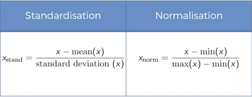
Standardization will put all the values of the feature in the range of [-3, 3].

Normalization will put all the values of the feature in the range of [0, 1].

So, which one to choose?

Well, normalization is recommended to use when you have a normal distribution in most of your features. This is very useful only for a specific case.
Standardization is more of a general case. It works all the time.

So, let's go for Standardization. To do this, we have to import the class StandardScaler from the Scikit library.

from sklearn.preprocessing import StandardScaler

#creating an object of that class
sc = StandardScaler()

The process is now intuitive and straightforward.

We have to fit and transform the X_train .

Note that the StandardScaler must be first fit and transform the training set but it must only transform the test set. This is done to prevent information about the distribution of the test set from leaking into the model.

X_train = sc.fit_transform(X_train)
X_test = sc.transform(X_test)

Depending on the Model or the dataset that you use, you might not have to go through all of the steps outlined above.

There you go! The above steps form the general outline for preprocessing the data before it can be pushed to any Machine Learning model.
So, this is how you can convert a raw dataset into a useful dataset.