
Photo by Luke Chesser on Unsplash
Performing ad hoc analysis is a daily part of life for most data scientists and analysts on operations teams.
They are often held back by not having direct and immediate access to their data because the data might not be in a data warehouse or it might be stored across multiple systems in different formats.
This typically means that a data engineer will need to help develop pipelines and tables that can be accessed in order for the analysts to do their work.
However, even here there is still a problem.
Data engineers are usually backed up with the amount of work they need to do, and often data for ad hoc analysis might not be a priority. This leads to analysts and data scientists either doing nothing or finagling their own data pipeline. This takes their time away from what they should be focused on.
Even if data engineers could help develop pipelines, the time required for new data to get through the pipeline could prevent operations analysts from analyzing data as it happens.
Getting access to data was, and honestly is still, a major problem in large companies.
Luckily, there are lots of great tools today to fix this. To demonstrate, we'll be using a free online data set that comes from Citi Bike in New York City, as well as S3, DynamoDB, and Rockset, a real-time cloud data store.
Citi Bike Data, S3, and DynamoDB
To set up this data, we'll be using the CSV data from Citi Bike ride data as well as the station data.
We'll be loading these data sets into two different AWS services. Specifically, we will be using DynamoDB and S3.
This will allow us to demonstrate the fact that sometimes it can be difficult to analyze data from both of these systems in the same query engine. In addition, the station data for DynamoDB is stored in JSON format which works well with DynamoDB. This is also because the station data is closer to live and seems to update every 30 seconds to one minute, whereas the CSV data for the actual bike rides is updated once a month. We will see how we can bring this near-real-time station data into our analysis without building out complicated data infrastructure.
Having these data sets in two different systems will also demonstrate where tools can come in handy. Rockset, for example, has the ability to easily join across different data sources such as DynamoDB and S3.
For a data scientist or analyst, this can make it easier to perform ad hoc analysis without needing to have the data transformed and pulled into a data warehouse first.
That being said, let's start looking into this Citi Bike data.
Loading Data Without a Data Pipeline
The ride data is stored in a monthly file as a CSV, which means we need to pull in each file in order to get the whole year.
For those who are used to the typical data engineering process, you will need to set up a pipeline that automatically checks the S3 bucket for new data and then loads it into a data warehouse like Redshift.
The data would follow a similar path to the one laid out below.

Image source: SeattleDataGuy
This means you need a data engineer to set up a pipeline.
However, in this case, I didn't need to set up any sort of data warehouse. Instead, I just loaded the files into S3 and then Rockset treated it all as one table.
Even though there are three different files, Rockset treats each folder as its own table. Kind of similar to some other data storage systems that store their data in partitions that are just essentially folders.
Not only that, it didn't freak out when you added a new column to the end. Instead, it just nulled out the rows that didn't have said column. This is great because it allows for new columns to be added without a data engineer needing to update a pipeline.
Analyzing Citi Bike Data
Generally, a good way to start is just to simply plot data out to make sure it somewhat makes sense (just in case you have bad data).
We will start with the CSVs stored in S3, and we will graph out usage of the bikes month over month.

Ride data example

To start off, we will just graph the ride data from September 2019 to November 2019. Below is all you will need for this query.
select
    count(*),
        cast(cast(starttime as datetime) as date)
from
    bike_rides b
group by
        cast(cast(starttime as datetime) as date)
Taking that data, I plotted it. You can see reasonable usage patterns. If we really wanted to dig into this, we would probably look into what was driving the dips to see if there was some sort of pattern, but for now. we are just trying to see the general trend.

Let's say you want to load more historical data because this data seems pretty consistent.
Again, no need to load more data into a data warehouse. You can just upload the data into S3 and it will automatically be picked up.
You can look at the graphs below to see the history looking further back.

From the perspective of an analyst or data scientist, this is great because I didn't need a data engineer to create a pipeline to answer my question about the data trend.
Looking at the chart above, we can see a trend where fewer people seem to ride bikes in winter, spring, and fall, but it picks up for summer. This makes sense because I don't foresee many people wanting to go out when it's raining in NYC.
All in all, this data passes the gut check, so we will look at it from a few more perspectives before joining the data.
What is the distribution of rides on an hourly basis?
Our next question is what is the distribution of rides on an hourly basis.
To answer this question, we need to extract the hour from the start time. This requires the EXTRACT function in SQL. Using that hour, you can then average it regardless of the specific date. Our goal is to see the distribution of bike rides.
Select
    EXTRACT(
        hour
        FROM
            cast(starttime as datetime)
    ),
    count(*)
from
    bike_rides
group by
    EXTRACT(
        hour
        FROM
            cast(starttime as datetime)
    )
We aren't going to go through every step we took from a query perspective, but you can look at the query and the chart below.
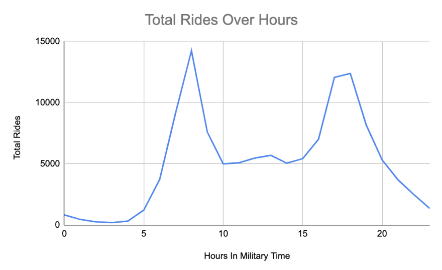
As you can see, there is clearly a trend to when people ride bikes. Specifically, there are surges in the morning and then again at night. This can be useful when it comes to knowing when it might be a good time to do maintenance or when bike racks are likely to run out.
But perhaps there are other patterns underlying this specific distribution.
What time do different riders use bikes?
Continuing on this thought, we also wanted to see if there were specific trends per rider types. This data set has two rider types: three-day customer passes and annual subscriptions.
We kept the hour extract and added in the ride type field.
Looking below at the chart, we can see that the trend for hours seems to be driven by the subscriber customer type.
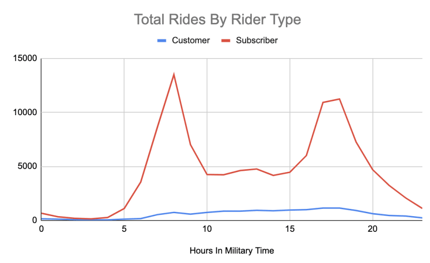
However, if we examine the customer rider type, we actually have a very different rider type. Instead of having two main peaks, there is a slow rising peak throughout the day that peaks around 17:00 to 18:00 (5--6 p.m.).
It would be interesting to dig into the why here. Is it because people who purchase a three-day pass are using it last minute? Or perhaps they're using it from a specific area. Does this trend look constant day over day?

Joining Data Sets Across S3 and DynamoDB
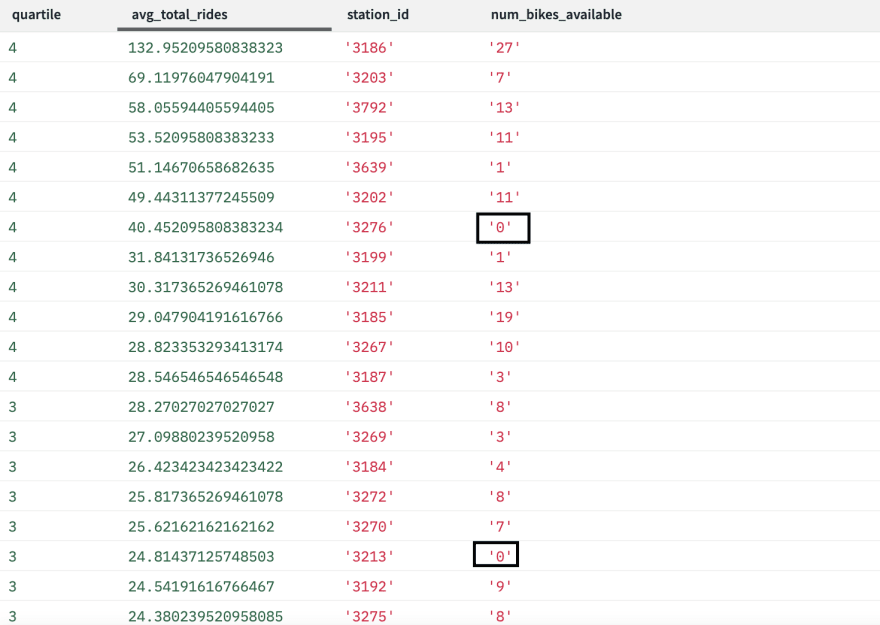
Finally, let's join in data from DynamoDB to get updates about the bike stations.

One reason we might want to do this is to figure out which stations have zero bikes left frequently and also have a high amount of traffic. This could be limiting riders from being able to get a bike because when they go for a bike, it's not there. This would negatively impact subscribers who might expect a bike to exist.
Below is a query that looks at the average rides per day per start station. We also added in a quartile just so we can look into the upper quartiles for average rides to see if there are any empty stations.
We listed out the output below, and as you can see, there are two stations currently empty that have high bike usage in comparison to the other stations. We would recommend tracking this over the course of a few weeks to see if this is a common occurrence. If it was, then Citi Bike might want to consider adding more stations or figuring out a way to reposition bikes to ensure customers always have rides.
Select NTILE(4) over (order by rn),
avg_total_rides,
station_id,
num_bikes_available
from
(
        select
            row_number() over (order by avg_total_rides desc) rn,
            t1.station_id,
            avg_total_rides,
            num_bikes_available
        from
            (
                select
                    avg(total_rides) avg_total_rides,
                    station_id
                from
                    (
                        select
                            sum(total_rides) total_rides,
                            start_date,
                            c."start station id" station_id
                        from
                            (
                                select
                                    cast(cast(starttime as datetime) as date) start_date,
                                    1 total_rides,
                                    b."start station id"
                                from
                                    bike_rides b
                            ) c
                        group by
                            start_date,
                            c."start station id"
                    ) d
                group by
                   station_id
            ) t1
            join (
                select
                    distinct station_id,
                    b.num_bikes_available
As operations analysts, being able to track live which high-usage stations are low on bikes can provide the ability to better coordinate teams that might be helping to redistribute bikes around town.
Rockset's ability to read data from an application database such as DynamoDB live can provide direct access to the data without any form of data warehouse. This avoids waiting for a daily pipeline to populate data. Instead, you can just read this data live.
Live Ad Hoc Analysis for Better Operations
Whether you're a data scientist or data analyst, the need to wait on data engineers and software developers to create data pipelines can slow down ad hoc analysis. Especially as more and more data storage systems are created, it just further complicates the work of everyone who manages data.
Thus, being able to easily access, join, and analyze data that isn't in a traditional data warehouse can prove to be very helpful and can lead to quick insights like the one about empty bike stations.
If you want to read more:
Airbnb's Airflow Vs Spotify's Luigi
Automating File Loading Into SQL Server With Python And SQL
5 Skills Every Software Engineer Needs Based Off Of A Job Description
The Top 10 Big Data Courses, Hadoop, Kafka And Spark
Data Science Use Cases That Are Improving the Finance Industry

Oldest comments (0)