Introduction to the Join Ordering Problem

A typical database may execute an SQL query in multiple ways, depending on the selected operators' order and algorithms. One crucial decision is the order in which the optimizer should join relations. The difference between optimal and non-optimal join order might be orders of magnitude. Therefore, the optimizer must choose the proper order of joins to ensure good overall performance. In this blog post, we define the join ordering problem and estimate the complexity of join planning.

Example

Consider the TPC-H schema. The customer may have orders. Every order may have several positions defined in the lineitem table. The customer table has 150,000 records, the orders table has 1,500,000 records, and the lineitem table has 6,000,000 records. Intuitively, every customer places approximately ten orders, and every order contains four positions on average.

Suppose that we want to retrieve all lineitem positions for all orders placed by the given customer:

SELECT 
  lineitem.*
FROM 
  customer,
  orders,
  lineitem
WHERE
  c_custkey = ? 
  AND c_custkey = o_custkey
  AND o_orderkey = l_orderkey

Assume that we have a cost model where an operator's cost is proportional to the number of processed tuples.

We consider two different join orders. We can join customer with orders and then with lineitem. This join order is very efficient because most customers are filtered early, and we have a tiny intermediate relation.

Alternatively, we can join orders with lineitem and then with customer. It produces a large intermediate relation because we map every lineitem to an order only to discard most of the produced tuples in the second join.

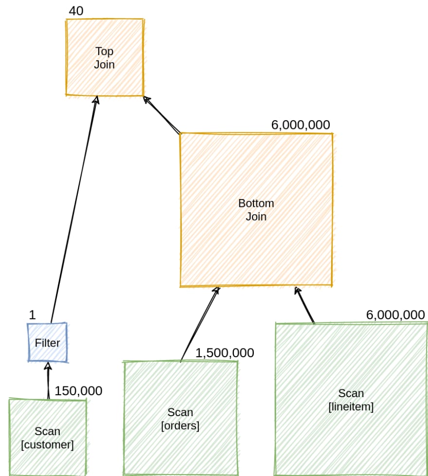
The two join orders produce plans with very different costs. The first join strategy is highly superior to the second.

Search Space

A perfect optimizer would need to construct all possible equivalent plans for a given query and choose the best plan. Let's now see how many options the optimizer would need to consider.

We model an n-way join as a sequence of n-1 2-way joins that form a full binary tree. Leaf nodes are original relations, and internal nodes are join relations. For 3 relations there are 12 valid join orders:

We count the number of possible join orders for N relations in two steps. First, we count the number of different orders of leaf nodes. For the first leaf, we choose one of N relations; for the second leaf, we choose one of remaining N-1 relations, etc. This gives us N! different orders.

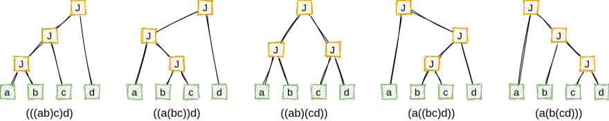
Second, we need to calculate the number of all possible shapes of a full binary tree with N leaves, which is the number of ways of associating N-1 applications of a binary operator. This number is known to be equal to Catalan number C(N-1). Intuitively, for the given fixed order of N leaf nodes, we need to find the number of ways to set N-1 pairs of open and close parenthesis. E.g., for the four relations [a,b,c,d], we have five different parenthesizations:

Multiplying the two parts, we get the final equation:

Performance

The number of join orders grows exponentially. For example, for three tables, the number of all possible join plans is 12; for five tables, it is 1,680; for ten tables, it is 17,643,225,600. Practical optimizers use different techniques to ensure a good enough performance of the join enumeration.

First, optimizers might use caching to minimize memory consumption. Two widely used techniques are dynamic programming and memoization.

Second, optimizers may use various heuristics to limit the search space instead of doing an exhaustive search. A common heuristic is to prune the join orders that yield cross-products. While good enough in the general case, this heuristic may lead to non-optimal plans, e.g., for some star joins. A more aggressive pruning approach is to enumerate only left- or right-deep trees. This significantly reduces planning complexity but degrades the plan quality even further. Probabilistic algorithms might be used (e.g., genetic algorithms or simulated annealing), also without any guarantees on the plan optimality.

Summary

In this post, we took a sneak peek at the join ordering problem and got a bird's-eye view of its complexity. In further posts, we will explore the complexity of join order planning for different graph topologies, dive into details of concrete enumeration techniques, and analyze existing and potential strategies of join planning in Apache Calcite. Stay tuned!

We are always ready to help you with your query optimizer design. Just let us know.