
Since ancient times, people have wondered about the uncertainty in the consequences of events. From the rolling of a dice, to the rotation of a card between two consoles, the concept of chance has developed. Randomness, as a definition, is not well founded, but we can simply call it the unpredictable state of a pile of events. For example, when a dice is rolled, its outcome cannot be predicted; the probability of coming double is 2 times more than coming 1.
In this article, we will examine the uncertainty starting from the recent past. Finally, we will consider the case of estimation with some regression models. Before we get started, let's examine our article in short headlines:
- Summary
- What is Randomness?
- Is it Predictable?
- Application
- Result
Summary
Randomness is not an outcome in itself. The result of the heads and tails is chaotic, not random. (See: Chaos Theory) It is an indication that we do not have instruments that can measure its randomness. The center of gravity of a metal coin is not clear due to the patterns on it. This money affects the result of situations such as being thrown from any side, shooting angle. The presence of too many variables on the result does not make it possible to estimate it completely in practice. I would like to underline that it is not impossible in theory.
What is Randomness?
The concept of randomness is a measure of uncertainty. It is not possible to catch randomness, except in the quantum state, which I will mention shortly. I mentioned the reason for this. It is practically impossible to find all the variables separately and calculate the result. To give an example, let's want to choose between objects with the same properties; we cannot seek pure randomness in this choice. Because we interpret within a stack of probabilities, more simply, we can predict the result with some accuracy.
You are familiar that in the microuniverse we call the subatomic level, we cannot apply a number of laws. The reason is the uncertainty, that is, the quantum state. Radioactive materials are made up of atoms that decay over time. The atoms that decay break down into smaller atoms. Scientifically, the probability of the atom to decay in a certain time interval can be calculated, but it is not possible to predict which atom is the next one to decay. "God doesn't roll dice!" he said. In reference to this statement, he mentioned that although the methods used are of great benefit in theory, they are not a good option to bring him closer to his secret. Said god is a philosophical god defined by Einstein himself.
Is it Predictable?
If you have managed to come up to this section, you can interpret the answer to the question yourself. Except for the quantum state, which we call a special case, predictions can be made about the distribution of results within the frame of probability. For the predictable situation, I would like to point out that it can be predicted in a very unrealistic way when the variables in the chaotic situation I mentioned earlier are ignored.
We gave our examples physically, but can random numbers be generated in computer environment? The short answer is that random generation cannot be made. It can be determined as a result of complex algorithms. I want to emphasize that it has been determined; The algorithms used work deterministically. Whatever the output is, it is certain.
Application
We will construct the pseudo-randomness case with the Python language and discuss its predictability. Since this part is for the fancier, you can skip to the conclusion part. Let's get to know the data set:

We have 5 'independent' variables: gender, age, number of monthly entries to the application, the number of monthly purchases, the averages of these purchases, and finally the conclusion part that we expect to stop applying. However, in our experiment; We have a total of 11 'independent' variables to make the entry, number of purchases and the average 3 each. The value we predict will leave is the dependent variable.
import random
import json
import pandas as pd
import numpy as np
import matplotlib.pyplot as plt
import pandas as pd

from sklearn.model_selection import train_test_split
from sklearn.preprocessing import StandardScaler
from sklearn.metrics import confusion_matrix
from sklearn.svm import SVC
from sklearn.linear_model import LogisticRegression
from sklearn.neighbors import KNeighborsClassifier
from sklearn.naive_bayes import GaussianNB
from sklearn.tree import DecisionTreeClassifier
from sklearn.ensemble import RandomForestClassifier
from sklearn.linear_model import LinearRegression


def jsonToCSV(numberOfDatas):
    name = ["data" + str(numberOfDatas[i]) for i in range(len(numberOfDatas))] #filenames = data + numberofdata's items
    fig, axs = plt.subplots(len(numberOfDatas)) #row numbers
    fig.suptitle('Epic Prediction')
    plt.setp(axs, yticklabels = ['SVC','LR','KN',"GNB",'DT',"RF"]) #label names
    y_pos = np.arange(len(['SVC','LR','KN',"GNB",'DT',"RF"])) #customizations
    fig.tight_layout()#customizations
    for i in range(len(name)): #We will generate random numbers as many as the element in the list numberOfDatas
        axs[i].set_yticks(y_pos+1)
        def gender():
            genderBinary = random.randint(0,1)
            return genderBinary
        def age():
            ageRandom = random.randint(18,65)
            return ageRandom

        def enteries():
            enteriesRandom = random.randint(0,300)
            return enteriesRandom

        def purchases():
            purchasesRandom = random.randint(1,100)
            return purchasesRandom

        def purchasesAv():
            purchasesAvRandom = random.randint(10,1500)
            return purchasesAvRandom

        def isLeave():
            isLeaveRandom = random.randint(0,1)
            return isLeaveRandom

        limit,index = 0,0
        dicts = {}
        while True:
            dicts[str(index)] = [gender(),
            age(),
            enteries(),enteries(),enteries(),
            purchases(),purchases(),purchases(),
            purchasesAv(),purchasesAv(),purchasesAv(),
            isLeave()]
            index +=1
            limit +=1
            if limit == numberOfDatas[i]:
                break

        with open(f'{name[i]}.json', 'w') as outfile: #We saved it in document datax.json (x = numberofdata's items)
            json.dump(dicts, outfile)

        df = pd.read_json(rf'{name[i]}.json')
        df.T.to_csv (rf'{name[i]}.csv', index = None) #We converted it to csv document. + transpose

        dataset = pd.read_csv(f'{name[i]}.csv') #we separated it as dependent independent variable.
        allOfThem= dataset.iloc[:,1:11].values
        willPredict = dataset.iloc[:,11:12].values

        X_train, X_test, y_train, y_test = train_test_split(allOfThem, willPredict, test_size = 0.25, random_state = 3)

        sc = StandardScaler()
        X_train = sc.fit_transform(X_train)
        X_test = sc.transform(X_test)
        """
        confusion matrix results
        [A B
         C D]
        Accuracy = (A+D/A+B+C+D ) * 100 => %bla bla
        """

        classifier = SVC(kernel = 'sigmoid', random_state = 4)
        classifier.fit(X_train, y_train)
        y_pred = classifier.predict(X_test)
        cm_SVC = confusion_matrix(y_test, y_pred)
        cm_SVC_C = (cm_SVC[0][0]+cm_SVC[1][1])/len(y_test)*100
        #print("SVC: %",cm_SVC_C)

        logr = LogisticRegression(random_state=3)
        logr.fit(X_train,y_train)
        y_pred = logr.predict(X_test)
        cm_LR = confusion_matrix(y_test, y_pred)
        cm_LR_C = (cm_LR[0][0]+cm_LR[1][1])/len(y_test)*100
        #print("LR: %",cm_LR_C)

        knn = KNeighborsClassifier(n_neighbors=11, metric='minkowski')
        knn.fit(X_train,y_train)
        y_pred = knn.predict(X_test)
        cm_KNN = confusion_matrix(y_test,y_pred)
        cm_KNN_C = (cm_KNN[0][0]+cm_KNN[1][1])/len(y_test)*100
        #print("KN: %",cm_KNN_C)

        gnb = GaussianNB()
        gnb.fit(X_train, y_train)
        y_pred = gnb.predict(X_test)
        cm_GNB = confusion_matrix(y_test,y_pred)
        cm_GNB_C = (cm_GNB[0][0]+cm_GNB[1][1])/len(y_test)*100
        #print("GaussianNB: %",cm_GNB_C)
        #print("Score:" , gnb.score(y_test, y_pred))

        dtc = DecisionTreeClassifier(criterion = 'entropy')
        dtc.fit(X_train,y_train)
        y_pred = dtc.predict(X_test)
        cm_DT = confusion_matrix(y_test,y_pred)
        cm_DT_C = (cm_DT[0][0]+cm_DT[1][1])/len(y_test)*100
        #print("DT: %",cm_DT_C)

        rfc = RandomForestClassifier(n_estimators=10, criterion = 'entropy')
        rfc.fit(X_train,y_train)
        y_pred = rfc.predict(X_test)
        cm_RF = confusion_matrix(y_test,y_pred)
        cm_RF_C= (cm_RF[0][0]+cm_RF[1][1])/len(y_test)*100
        #print("RF: %",cm_RF_C)

        listOfResults_X = [round(cm_SVC_C,4),round(cm_LR_C,4),round(cm_KNN_C,4),round(cm_GNB_C,4),round(cm_DT_C,4),round(cm_RF_C,4)]#we rounded the numbers
        listOfResults_Y = [1,2,3,4,5,6]

        axs[i].barh(1,cm_SVC_C,height = 1,color = "darkcyan", label='SVC')
        axs[i].barh(2,cm_LR_C,height = 1,color = "darkturquoise", label='LR')
        axs[i].barh(3,cm_KNN_C,height = 1,color = "steelblue", label='KN')
        axs[i].barh(4,cm_GNB_C, height = 1,color = "palevioletred", label='GNB')
        axs[i].barh(5,cm_DT_C, height = 1,color = "darkmagenta", label='DT')
        axs[i].barh(6,cm_RF_C,height = 1,color = "rosybrown", label='RF')

        for x in range(6):
            axs[i].text(x = listOfResults_X[x] , y = listOfResults_Y[x] - 0.25, s = listOfResults_X[x], size = 9)
        axs[i].set_title("The Number Of Data : " + str(numberOfDatas[i]))
        axs[i].set_xlabel('Prediction Rate')
        axs[i].set_ylabel('Regression Models')
    axs[-1].legend(loc=2)
    plt.show()

jsonToCSV([100,1000,5000]) #If you want, you can change these items.
Result
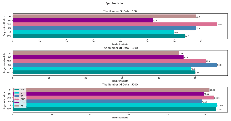
Since we entered the values of 100,1000 and 5000, we obtained 3 result graphs. In the case of low data numbers, the models are more predictable, while the higher this number, the lower the performance rate. First of all, we can make this comment. Next, we will focus on the fact that when the data increase, the rates of correct estimation decrease and the results of the regression models are close to each other. Why is it so low? Although it is low, how and why does it show results close to 50%?
In fact, we can interpret such low rates as the fact that there is no link between the data. Likewise, we can relate its convergence to 50% with the probability distributions I mentioned earlier. You can click here for the article on this topic.

Latest comments (0)