
Sparkify — Digital Music Service
Customer Churn Analysis & Prediction
Sparkify is a digital music service similar to Spotify and fizy. Many users make subscriptions, listen their favourite songs with free (with advertisement) or paid subscriptions, add friends or songs to their playlists etc. Users can also upgrade, downgrade or cancel your subscriptions in any time. Similar to all digital services and their subscriptions, member churn is the most important problem, so company should define model to identify customers who are potentially churn and make marketing offers to keep their subscriptions.
Business Problem: is that predicting potential customers who will churn from Sparkify digital music service.
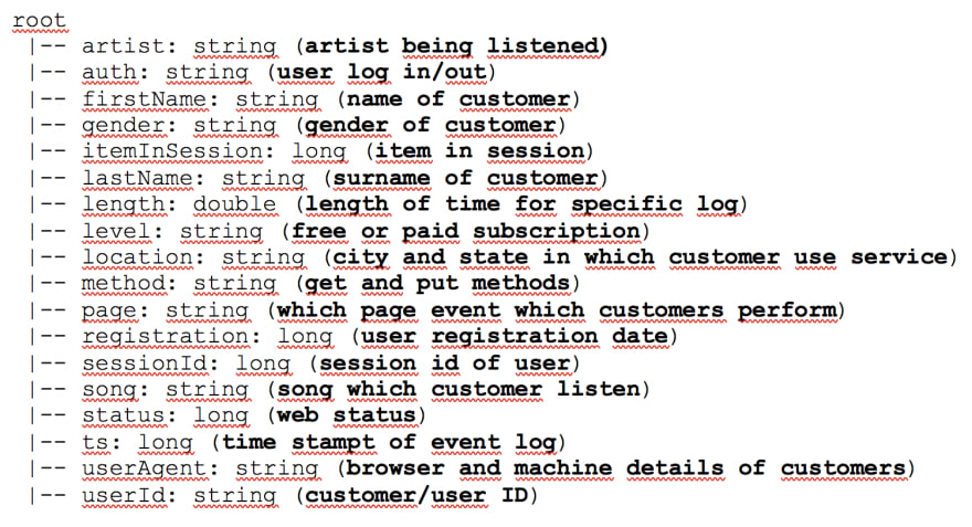
Datasets: Udacity provides mini dataset (128MB) and full dataset (12GB) including transactional log data of users in Sparkify. I have used mini dataset in Jupyter notebook to perform explanatory data analysis and implement model. Mini json dataset including 18 columns including 12 categorical columns (string) and 6 numerical columns (long and double) and 286.500 records.
After loading and preliminary observation of data above, I started to clean data:
1. Drop NaN and ‘ ‘ values (empty strings)
#Check missing values and '' data for each column.
print('Count of Missing Values for each Column')
for col in df.columns:
    missing_count = df.filter((df[col] == "") | df[col].isNull() | isnan(df[col])).count()
    print('{}: '.format(col), missing_count)

*There are 8.346 missing values for userId and other related columns (first name, last name etc.) These records should be dropped, because userId is important column to define potential customers who churn. After cleaning, there are also 58.392 missing values for artist and song. However, they can be acceptable, because all Sparkify transaction in dataset is not related with play song in data.*
2. Convert “registration” and “ts” columns to human readable form to detect registration and page event log dates in mini dataset.
convert_ts = udf(lambda x: datetime.datetime.fromtimestamp(x / 1000.0).strftime("%Y-%m-%d %H:%M:%S"))
df_clean = df_clean.withColumn('page_event_time', convert_ts('ts'))
df_clean = df_clean.withColumn('registration_time', convert_ts('registration'))
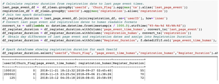
Furthermore, I will create “register_duration” column to calculate customer lifetime between registration and last page event dates. It will be also used as feature in modelling.
3. Split location columns to define city and state in different columns.
import pyspark.sql.functions as f
split_col = f.split(df_clean['location'], ',')
df_clean = df_clean.withColumn('City', split_col.getItem(0))
df_clean = df_clean.withColumn('State', split_col.getItem(1))

After cleaning data, there are 278.154 records and 22 columns including new columns: page_event_time, registration_time, City and State.
After these data cleaning and type conversion, I created columns;
“Register_Duration”: day difference of “page_event_date” and “registration_time”
“Churn_Flag” column: using “Cancellation Confirmation” events of page column to define churn as “1”

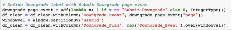
- “Downgrade_Event”: Using “Submit Downgrade” events of page column to define downgrade as “1”.
Exploratory Data Analysis
After cleaning data, I performed some exploratory data analysis.
1. There are 121 male and 104 female users in data frame. It is approximately balanced data according to gender.
df_clean.createOrReplaceTempView("Sparkify_df_clean")
spark.sql('''
        SELECT gender,COUNT(DISTINCT userId) AS user_counts
        FROM Sparkify_df_clean
        GROUP BY gender
        ORDER BY user_counts DESC
''').show()
+------+-----------+

|gender|user_counts|

+------+-----------+

|     M|        121|

|     F|        104|

+------+-----------+
2. Majority of page event data is composed of *“NextSong” (80% of data: 228.108 / 278.154)***
Furthermore, “Cancel Confirmation” page event is also 52 and this event was used to define churn.
spark.sql('''
        SELECT page,COUNT(userId) AS user_counts
        FROM Sparkify_df_clean
        GROUP BY page
        ORDER BY user_counts DESC
''').show()
+--------------------+-----------+

|                page|user_counts|

+--------------------+-----------+

|            **NextSong|     228108**|

|           Thumbs Up|      12551|

|                Home|      10082|

|     Add to Playlist|       6526|

|          Add Friend|       4277|

|         Roll Advert|       3933|

|              Logout|       3226|

|         Thumbs Down|       2546|

|           Downgrade|       2055|

|            Settings|       1514|

|                Help|       1454|

|             Upgrade|        499|

|               About|        495|

|       Save Settings|        310|

|               Error|        252|

|      Submit Upgrade|        159|

|    Submit Downgrade|         63|

|              Cancel|         52|

|**Cancellation Conf...|         52**|

+--------------------+-----------+
3. There are 195 free and 165 paid account in this dataset. There are 225 userIds in dataframe, so it shows that 135 users have changed their account level.
spark.sql('''
        SELECT level,COUNT(DISTINCT userId) AS user_counts
        FROM  Sparkify_df_clean
        GROUP BY level
        ORDER BY user_counts DESC
''').show()
+-----+-----------+

|level|user_counts|

+-----+-----------+

| free|        195|

| paid|        165|

+-----+-----------+
4. I checked city and state distribution in which customers locate. Majority of users are in CA, TX, NY-NJ-PA, FL states. Furthermore, LA-Long Beach and NY City are the top cities. However, there was no extraordinary bias in location in mini dataset.
# City distribution of users is showed below. LA and NY are top cities.
city_dist = spark.sql('''
        SELECT City,COUNT(DISTINCT userId) AS user_counts
        FROM Sparkify_df_clean
        GROUP BY City
        ORDER BY user_counts DESC
''').toPandas()

# Plot graph for distribution
sns.set(rc={'figure.figsize':(30,50)})
plt.title('City Distribution of Users', size=20)
barplot = sns.barplot(x = 'user_counts', y = 'City', data = city_dist, palette = 'dark')
plt.show()
# Majority of Users are in CA, TX, NY-NJ-PA, FL states.
state_dist = spark.sql('''
        SELECT State,COUNT(DISTINCT userId) AS user_counts
        FROM Sparkify_df_clean
        GROUP BY State
        ORDER BY user_counts DESC
''').toPandas()

# Plot graph for distribution
sns.set(rc={'figure.figsize':(30,50)})
plt.title('State Distribution of Users', size=20)
barplot = sns.barplot(x = 'user_counts', y = 'State', data = state_dist, palette = 'dark')
plt.show()


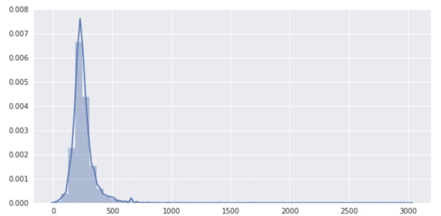
5. I checked length of time for current row of specific log and show distribution of length of event logs. Majority of length is between 0 and 500 minutes.
length_data = spark.sql('''
        SELECT length
        FROM Sparkify_df_clean
''')
sns.set(rc={'figure.figsize':(10,5)})
sns.distplot(length_data.toPandas().dropna());
6.There are 52 users cancelled their service and 49 users downgraded their service in dataset.
df_clean.createOrReplaceTempView("Sparkify_df_clean")
spark.sql('''
        SELECT Churn_Flag,COUNT(DISTINCT userId) AS user_counts
        FROM  Sparkify_df_clean
        GROUP BY Churn_Flag
        ORDER BY user_counts DESC
''').show()

df_clean.createOrReplaceTempView("Sparkify_df_clean")
spark.sql('''
        SELECT Downgrade_Flag,COUNT(DISTINCT userId) AS user_counts
        FROM  Sparkify_df_clean
        GROUP BY Downgrade_Flag
        ORDER BY user_counts DESC
''').show()

7.While taking into “gender” into regard, I checked churn and play next song analysis. Male customers who churned played slightly more than female customers. On the other hand, female customers who did not churn, play more song then male customers.
Same analysis was also performed for “Thumbs Up” page event. Similar results were also observed.
df_clean.createOrReplaceTempView("Sparkify_df_clean")
cust_positive_lifetime_1 = spark.sql('''
        SELECT  gender, Churn_Flag, COUNT(userId) AS user_counts
        FROM  Sparkify_df_clean
        WHERE page == "NextSong"
        GROUP BY gender, Churn_Flag
        ORDER BY user_counts DESC
''').toPandas()
sns.set(rc={'figure.figsize':(10,5)})
ax = sns.barplot(x='Churn_Flag', y='user_counts', hue='gender', data=cust_positive_lifetime_1)
plt.xlabel('Customer Churn Flag - (0: No) (1: Yes)')
plt.ylabel('User Counts')
plt.legend(title='Gender', loc='best')
plt.title('Customer Listen Next Song Analysis: Churn vs. Gender')
sns.despine(ax=ax);

df_clean.createOrReplaceTempView("Sparkify_df_clean")
cust_positive_lifetime_2 = spark.sql('''
        SELECT  gender, Churn_Flag, COUNT(userId) AS user_counts
        FROM  Sparkify_df_clean
        WHERE page == "Thumbs Up"
        GROUP BY gender, Churn_Flag
        ORDER BY user_counts DESC
''').toPandas()
sns.set(rc={'figure.figsize':(10,5)})
ax = sns.barplot(x='Churn_Flag', y='user_counts', hue='gender', data=cust_positive_lifetime_2)
plt.xlabel('Customer Churn Flag - (0: No) (1: Yes)')
plt.ylabel('User Counts')
plt.legend(title='Gender', loc='best')
plt.title('Customer Thumbs Up Analysis: Churn vs. Gender')
sns.despine(ax=ax);

8. I also explored churn pattern according to gender and account level. According to analysis, male customers are more likely to churn than female customers. Furthermore, customers having paid account churned more than customers having free account.
# Explore churn pattern according to gender: Male customers are more likely to churn than female customers.
df_clean.createOrReplaceTempView("Sparkify_df_clean")
churn_gender_analysis_pd = spark.sql('''
        SELECT gender, Churn_Flag, COUNT( DISTINCT userId) AS user_counts
        FROM  Sparkify_df_clean
        GROUP BY  gender, Churn_Flag
        ORDER BY user_counts DESC
''').toPandas()
sns.set(rc={'figure.figsize':(10,5)})
ax = sns.barplot(x='Churn_Flag', y='user_counts', hue='gender', data=churn_gender_analysis_pd)
plt.xlabel('Customer Churn Flag - (0: No) (1: Yes)')
plt.ylabel('User Counts')
plt.legend(title='Gender', loc='best')
plt.title('Churn vs. Gender Analysis')
sns.despine(ax=ax);

# Explore churn pattern according to level (paid and free): Customers having paid account are more likely to churn than customers having free account.
df_clean.createOrReplaceTempView("Sparkify_df_clean")
churn_level_analysis_pd = spark.sql('''
        SELECT level, COUNT(DISTINCT userId) AS user_counts
        FROM  Sparkify_df_clean
        WHERE page == "Cancellation Confirmation"
        GROUP BY level
        ORDER BY user_counts DESC
''').toPandas()
sns.set(rc={'figure.figsize':(10,5)})
ax = sns.barplot(x='level', y='user_counts', data=churn_level_analysis_pd)
plt.xlabel('Customer Churn Flag - (0: No) (1: Yes)')
plt.ylabel('User Counts')
plt.legend(title='Level', loc='best')
plt.title('Churn vs. Level Analysis')
sns.despine(ax=ax);

9. Register duration (customer lifetime) of customers churned is less than customers who did not churn.
df_register_duration_pd = df_register_duration.toPandas()
ax = sns.boxplot(data=df_register_duration_pd, y='Churn_Flag', x='Register_Duration', orient='h')
plt.xlabel('Days Between Last Page Event and Registration')
plt.ylabel('Customer Churn Flag - (0: No) (1: Yes)')
plt.title('Registration Duration vs. Churn Analysis')
sns.despine(ax=ax);

10. I performed analysis total listened songs and average listened songs per session according to churn status of customers. Customers who churned normally listened less songs than customers who did not churn.
# Total number of song listened vs. Churn Analysis
# It shows that users churned listen less song.
df_clean.createOrReplaceTempView("Sparkify_df_clean")
churn_listenedsong_analysis_pd = spark.sql('''
        SELECT Churn_Flag, userID, sum(page_counts) AS sum_page_counts
        FROM
        (SELECT Churn_Flag, userId, count(page) AS page_counts
        FROM  Sparkify_df_clean
        WHERE page == "NextSong"
        GROUP BY Churn_Flag, userId)
        GROUP BY Churn_Flag, userID
''').toPandas()

ax = sns.boxplot(data=churn_listenedsong_analysis_pd, y='Churn_Flag', x='sum_page_counts', orient='h')
plt.xlabel('Total Number of Song Listened')
plt.ylabel('Customer Churn Flag - (0: No) (1: Yes)')
plt.title('Total Listened Song vs. Churn Analysis')
sns.despine(ax=ax);

# Average Number of song listened per session vs. Churn Analysis
# It shows that users churned listen less song per session.
df_clean.createOrReplaceTempView("Sparkify_df_clean")
churn_ses_listenedsong_analysis_pd = spark.sql('''
        SELECT Churn_Flag, userID, avg(page_counts) AS avg_page_counts
        FROM
        (SELECT Churn_Flag, userId, sessionid, count(page) AS page_counts
        FROM  Sparkify_df_clean
        WHERE page == "NextSong"
        GROUP BY Churn_Flag, userId, sessionid)
        GROUP BY Churn_Flag, userID
''').toPandas()

ax = sns.boxplot(data=churn_ses_listenedsong_analysis_pd, y='Churn_Flag', x='avg_page_counts', orient='h')
plt.xlabel('Average Number of Song Listened Per Session')
plt.ylabel('Customer Churn Flag - (0: No) (1: Yes)')
plt.title('Average Listened Song per Session vs. Churn Analysis')
sns.despine(ax=ax);

11. I performed thumbs up and down events according to churn status of customers. Customers who churned normally less thumbs up than customers who did not churn.
# Number of thumbs up vs. Churn Analysis: It shows that users churned make less thumbs up.
df_clean.createOrReplaceTempView("Sparkify_df_clean")
thumbs_up_analysis_pd = spark.sql('''
        SELECT Churn_Flag, userId, count(page) AS page_counts
        FROM  Sparkify_df_clean
        WHERE page == "Thumbs Up"
        GROUP BY Churn_Flag, userId
''').toPandas()

ax = sns.boxplot(data=thumbs_up_analysis_pd, y='Churn_Flag', x='page_counts', orient='h')
plt.xlabel('Number of Thumbs Up')
plt.ylabel('Customer Churn Flag - (0: No) (1: Yes)')
plt.title('Number of Thumbs Up vs. Churn Analysis')
sns.despine(ax=ax);

# Number of thumbs down vs. Churn Analysis: It shows that the number of thumbs down is similar according to churn flag.
df_clean.createOrReplaceTempView("Sparkify_df_clean")
thumbs_down_analysis_pd = spark.sql('''
        SELECT Churn_Flag, userId, count(page) AS page_counts
        FROM  Sparkify_df_clean
        WHERE page == "Thumbs Down"
        GROUP BY Churn_Flag, userId
''').toPandas()

ax = sns.boxplot(data=thumbs_down_analysis_pd, y='Churn_Flag', x='page_counts', orient='h')
plt.xlabel('Number of Thumbs Down')
plt.ylabel('Customer Churn Flag - (0: No) (1: Yes)')
plt.title('Number of Thumbs Down vs. Churn Analysis')
sns.despine(ax=ax);

12. Finally, I performed analysis add playlist and friend page transactions according to churn status. Customers who churned normally perform less “add friend” and “add playlist” transactions than customers who did not churn.
# Number of Add Playlist vs. Churn Analysis: It shows that users churned make less "add playlist"
df_clean.createOrReplaceTempView("Sparkify_df_clean")
playlist_analysis_pd = spark.sql('''
        SELECT Churn_Flag, userId, count(page) AS page_counts
        FROM  Sparkify_df_clean
        WHERE page == "Add to Playlist"
        GROUP BY Churn_Flag, userId
''').toPandas()

ax = sns.boxplot(data=playlist_analysis_pd, y='Churn_Flag', x='page_counts', orient='h')
plt.xlabel('Number of Add Playlist')
plt.ylabel('Customer Churn Flag - (0: No) (1: Yes)')
plt.title('Number of Add Playlist vs. Churn Analysis')
sns.despine(ax=ax);

# Number of Add Friend vs. Churn Analysis: It shows that users churned make less "add friend"
df_clean.createOrReplaceTempView("Sparkify_df_clean")
addfriend_analysis_pd = spark.sql('''
        SELECT Churn_Flag, userId, count(page) AS page_counts
        FROM  Sparkify_df_clean
        WHERE page == "Add Friend"
        GROUP BY Churn_Flag, userId
''').toPandas()

ax = sns.boxplot(data=addfriend_analysis_pd, y='Churn_Flag', x='page_counts', orient='h')
plt.xlabel('Number of Add Friend')
plt.ylabel('Customer Churn Flag - (0: No) (1: Yes)')
plt.title('Number of Add Friend vs. Churn Analysis')
sns.despine(ax=ax);

Feature Engineering
After defining churn label and exploratory data analysis explained above, I calculated feature metrics below to solve problem (predicting potential customers who will churn.)
These 10 features are
Registration duration (customer lifetime — important for loyalty),
Total number of songs listened
Average number songs listened per session
The number of thumbs up
The number of thumbs down
The number of add friends
The number of add playlist
Total length of listening
Gender
Account level (paid or free)
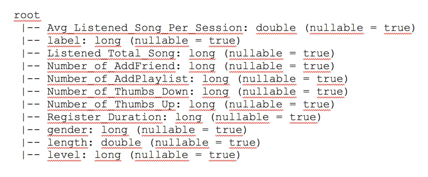
These features will serve as inputs and outputs for designed machine learning model in next section. Except “label” (churn label), there are 10 feature metrics in calculated dataset used in models.
# Read model data from json file.
model_data = spark.read.json('df_final_model_data.json')
# change column name Churn_Label to label
model_data = model_data.withColumnRenamed("Churn_Label","label")
# Check columns and shape
model_data.printSchema()
model_data.toPandas().shape
Modelling
For this step of my project, I will be building 3 base models that could possibly be used for predicting churn. Since churn is a simple churned/not-churned value, I can leverage classification models. The models I will be building are below:
Logistic Regression Model -(https://spark.apache.org/docs/latest/api/python/pyspark.ml.html#pyspark.ml.classification.LogisticRegression)
Random Forest Model -
(http://spark.apache.org/docs/latest/ml-classification-regression.html#random-forest-regression)
GBT Classifier Model - (https://spark.apache.org/docs/latest/api/python/pyspark.ml.html#pyspark.ml.classification.GBTClassifier)
From these models I will be providing their results and evaluating their Accuracy and F1-Score. It is important for me to understand when my models are being as accurate as possible when determining when one of my users will possibly be churning and thus this is something that I will check against all models.
However, Accuracy is not everything thus I must also make sure to not have a model that will potentially tell me a lot more users could possibly be churning when in reality they may not or there may be too many users showing possible churn.
This could potentially lead to time wasted on users that are not churning and could mean extra costs for Sparkify. To balance this, I will be evaluating and optimizing the F1-Score which is a function of Precision and Recall to help give me the right balanced model.
Logistic Regression Metrics:
# import time to calculate model training duration (seconds)
from time import time

# 1. Logistic Regression

# initialize classifier, set evaluater and build paramGrid
lr = LogisticRegression(maxIter=10)
f1_evaluator = MulticlassClassificationEvaluator(metricName='f1')
paramGrid = ParamGridBuilder().build()
crossval_lr = CrossValidator(estimator=lr, evaluator=f1_evaluator, estimatorParamMaps=paramGrid,numFolds=3)

# Calculate time metric of model.
start_time = time()
cvModel_lr = crossval_lr.fit(train)
end_time = time()
cvModel_lr.avgMetrics
seconds = end_time- start_time

results_lr = cvModel_lr.transform(validation)

evaluator = MulticlassClassificationEvaluator(predictionCol="prediction")

print('Logistic Regression Metrics:')
print('Accuracy of model is : {}'.format(evaluator.evaluate(results_lr, {evaluator.metricName: "accuracy"})))
print('F1 score of model is :{}'.format(evaluator.evaluate(results_lr, {evaluator.metricName: "f1"})))
print('The training process of model took {} seconds'.format(seconds))
Accuracy of model is : 0.7887323943661971
F1 score of model is :0.7189395194697596
The training process of model took 4.507469654083252 seconds
Random Forest Metrics:
# 2. Random Forest Classifier

# initialize classifier, set evaluater and build paramGrid
rf = RandomForestClassifier()
f1_evaluator = MulticlassClassificationEvaluator(metricName='f1')
paramGrid = ParamGridBuilder().build()
crossval_rf = CrossValidator(estimator=rf,estimatorParamMaps=paramGrid,evaluator=f1_evaluator,numFolds=3)

# Calculate time metric of model.
start_time = time()
cvModel_rf = crossval_rf.fit(train)
end_time = time()
cvModel_rf.avgMetrics
seconds = end_time- start_time

results_rf = cvModel_rf.transform(validation)

evaluator = MulticlassClassificationEvaluator(predictionCol="prediction")

print('Random Forest Metrics:')
print('Accuracy of model is : {}'.format(evaluator.evaluate(results_rf, {evaluator.metricName: "accuracy"})))
print('F1 score of model is :{}'.format(evaluator.evaluate(results_rf, {evaluator.metricName: "f1"})))
print('The training process of model took {} seconds'.format(seconds))
Accuracy of model is : 0.9014084507042254
F1 score of model is :0.8972171191399606
The training process of model took 4.879174709320068 seconds
Gradient Boosted Trees Metrics:
# 3. Gradient Boosting Trees

# initialize classifier, set evaluater and build paramGrid
gbt = GBTClassifier(maxIter=10,seed=42)
f1_evaluator = MulticlassClassificationEvaluator(metricName='f1')
paramGrid = ParamGridBuilder().build()
crossval_gbt = CrossValidator(estimator=gbt,estimatorParamMaps=paramGrid,evaluator=f1_evaluator,numFolds=3)

# Calculate time metric of model.
start_time = time()
cvModel_gbt = crossval_gbt.fit(train)
end_time = time()
cvModel_gbt.avgMetrics
seconds = end_time- start_time

results_gbt = cvModel_gbt.transform(validation)

evaluator = MulticlassClassificationEvaluator(predictionCol="prediction")

print('Gradient Boosted Trees Metrics:')
print('Accuracy of model is : {}'.format(evaluator.evaluate(results_gbt, {evaluator.metricName: "accuracy"})))
print('F1 score of model is :{}'.format(evaluator.evaluate(results_gbt, {evaluator.metricName: "f1"})))
print('The training process of model took {} seconds'.format(seconds))
Accuracy of model is : 0.8450704225352113
F1 score of model is :0.8430847520275758
The training process of model took 21.43347477912903 seconds
*Why Random Forrest Model is best for our scenario:*
First of all we used f1-score to select our final model because our problem is classification one and f1-score can help us to find the balance between accuracy and recall. Higher the f1-score the more perfect our model will be as false negative and false positive will be less.
Here Random Forrest has best f1-score that's why I choose it for the next steps.
Then, I have applied hyperparameter tuning based on f1 score :
# Optimizing Hyperparameters in Random Forest Classification
clf = RandomForestClassifier()
numTrees=[20,75]
maxDepth=[10,20]
paramGrid = ParamGridBuilder().addGrid(clf.numTrees, numTrees).addGrid(clf.maxDepth, maxDepth).build()
crossval = CrossValidator(estimator = Pipeline(stages=[clf]),
                         estimatorParamMaps = paramGrid,
                         evaluator = MulticlassClassificationEvaluator(metricName='f1'),
                         numFolds = 3)

cvModel_rf = crossval.fit(train)
predictions = cvModel_rf.transform(test)

evaluator = MulticlassClassificationEvaluator(metricName='f1')
f1_score = evaluator.evaluate(predictions.select(col('label'), col('prediction')))
print('The F1 score is {:.2%}'.format(f1_score))

bestPipeline = cvModel_rf.bestModel

print('Best parameters : max depth:{}, num Trees:{}'.format(bestPipeline.stages[0].getOrDefault('maxDepth'), bestPipeline.stages[0].getNumTrees))
After execution hyperparameter tuning; best parameters and f1-score were listed below:
The F1 score is 91.39%
Best parameters : max depth:10, num Trees:75
Finally, Random Forrest Classifier (RF) Model is executed with best parameters (max depth:10, num Trees:75), I obtained higher accuracy and f1-score values below:
# Best Model: Random Forrest Model with max depth:10, num Trees:75 parameters
rf_best = RandomForestClassifier(numTrees=75, maxDepth=10)
rf_best_model = rf_best.fit(train)
result = rf_best_model.transform(test)
evaluator = MulticlassClassificationEvaluator(predictionCol="prediction")
print('Random Forrest Model - Test Metrics with best parameters:')
print('Accuracy of model is :  {}'.format(evaluator.evaluate(result, {evaluator.metricName: "accuracy"})))
print('F1 score of model is : {}'.format(evaluator.evaluate(result, {evaluator.metricName: "f1"})))

Accuracy and f1 score are very good. However, it should not be forgotten that my dataset may not be representing all customer base, I used mini — sized dataset. In real world and big data set, I think that 80% accuracy ratio is very good.
I have also calculated feature importance in predicting customer churn. I observe that register_duration (days — customer lifetime), number of thumbs down and average listened songs per session are top 3 important features while predicting churn.
# Features importance of Random Forrest Model
Feature_Importance_Scores = rf_best_model.featureImportances.values.tolist()
Feature_Importance_df = pd.DataFrame({'Feature_Importance_Scores': Feature_Importance_Scores, 'Features': columns})
plt.title('Features Importance Scores of Random Forrest Model')
sns.barplot(x='Feature_Importance_Scores', y='Features', data=Feature_Importance_df, color="blue")

Conclusion
In Udacity — Sparkify Project, I try to generate model predicting customer churn. While building a model to predict customer churn from a transactional user data of Sparkify, these steps have been completed:
Load mini json dataset file, clean data and make ready for explanatory data analysis.
Perform explanatory data analysis, define churn and try to determine features which will be used in model.
Define 10 features which will be used in model while predicting churn.
Select three models which are logistic regression, random forest and gradient boosting trees to compare model.
Select random forest model as the final model implemented for predicting final result and also fine-tuning its parameters. I obtained approximately 92% accuracy and 0.913 f1 score with this model.
Finally, I observed that register_duration (days), number of thumbs down and average listened songs per session are top 3 important features while predicting churn.
ML algorithms with Spark provides us to process big data, gain insight and develop actions from predictions. For this project, Sparkify can make marketing campaign to customers who will potentially churn to prevent higher churn rates.
Feature engineering is also very important to define correct metrics in prediction models. In this project, I thought and defined 10 numerical features having impact on churn. However, many metrics can also be added while working with big data to improve model. For instance, rolling advertisement, log out event can also be added into features. However, I obtained good accuracy and f1-score with existing mini dataset. Extra features can be also taken into account while working with big dataset.
References:
GitHub: https://github.com/ankit1797/Udacity-data-scientist-capstone-project

Top comments (1)
Now this thing can be done by a Churnfree you can check out this customer retention software.
This is best for the SaaS, eCommerce and membership business.
This will also help you in your app i will suggest you to once check out this.
It will help you in your business growth.