Use Advanced MySQL Operations to Analyze Python Web Scraper Data

Prerequisites

To follow this tutorial, you should have the following:

• Python 3.7 or newer.
• Arctype
• Basic understanding of SQL.
• A text editor.

Installing the required libraries

The libraries required for this tutorial are as follows:

• numpy — fundamental package for scientific computing with Python
• pandas — library providing high-performance, easy-to-use data structures, and data analysis tools
• requests — is the only Non-GMO HTTP library for Python, safe for human consumption. (love this line from official docs :D)
• BeautifulSoup — a Python library for pulling data out of HTML and XML files.

To install the libraries required for this tutorial, run the following commands below:

pip install numpy
pip install pandas
pip install requests
pip install bs4

Building the Python Web Scraper

Now that we have all the required libraries installed let’s get to building our web scraper.

Importing the Python libraries

 import numpy as np
 import pandas as pd
 import requests
 from bs4 import BeautifulSoup
 import json

Carrying Out Site Research

The first step in any web scraping project is researching the web page you want to scrape and learn how it works. That is critical to finding where to get the data from the site. For this tutorial, we'll be using http://understat.com.

We can see on the home page that the site has data for six European leagues. However, we will be extracting data for just the top 5 leagues(teams excluding RFPL).

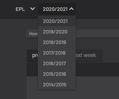
We can also notice that data on the site starts from 2014/2015 to 2020/2021. Let’s create variables to handle only the data we require.

# create urls for all seasons of all leagues
 base_url = 'https://understat.com/league'
 leagues = ['La_liga', 'EPL', 'Bundesliga', 'Serie_A', 'Ligue_1']
 seasons = ['2016', '2017', '2018', '2019', '2020']    

The next step is to figure out where the data on the web page is stored. To do so, open Developer Tools in Chrome, navigate to the Network tab, locate the data file (in this example, 2018), and select the “Response” tab. After executing requests, this is what we'll get.

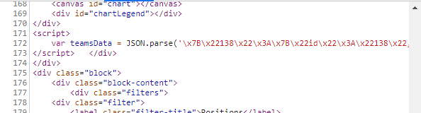
After looking through the web page's content, we discovered that the data is saved beneath the "script" element in the teamsData variable and is JSON encoded. As a result, we'll need to track down this tag, extract JSON from it, and convert it to a Python-readable data structure.

Decoding the JSON Data with Python

season_data = dict()
for season in seasons:
url = base_url+'/'+league+'/'+season
res = requests.get(url)
soup = BeautifulSoup(res.content, "lxml")
# Based on the structure of the webpage, I found that data is in the JSON variable, under <script> tags
scripts = soup.find_all('script')
string_with_json_obj = ''
# Find data for teams
for el in scripts:
if 'teamsData' in str(el):
string_with_json_obj = str(el).strip()
# strip unnecessary symbols and get only JSON data
ind_start = string_with_json_obj.index("('")+2
ind_end = string_with_json_obj.index("')")
json_data = string_with_json_obj[ind_start:ind_end]
json_data = json_data.encode('utf8').decode('unicode_escape')
#print(json_data)

After running the python code above, you should get a bunch of data that we’ve cleaned up.

Understanding the Scraper Data

When we start looking at the data, we realize it's a dictionary of dictionaries with three keys: id, title, and history. Ids are also used as keys in the dictionary's initial layer.

Therefore, we can deduce that history has information on every match a team has played in its own league (League Cup or Champions League games are not included).

After reviewing the first layer dictionary, we can begin to compile a list of team names.

# Get teams and their relevant ids and put them into separate dictionary
teams = {}
for id in data.keys():
teams[id] = data[id]['title']

We see that column names frequently appear; therefore, we put them in a separate list. Also, look at how the sample values appear.

columns = []
# Check the sample of values per each column
values = []
for id in data.keys():
columns = list(data[id]['history'][0].keys())
values = list(data[id]['history'][0].values())
break

Now let’s get data for all teams. Uncomment the print statement in the code below to print the data to your console.

# Getting data for all teams
dataframes = {}
for id, team in teams.items():
teams_data = []
for row in data[id]['history']:
teams_data.append(list(row.values()))
df = pd.DataFrame(teams_data, columns=columns)
dataframes[team] = df
# print('Added data for {}.'.format(team))

After you have completed this code, we will have a dictionary of DataFrames with the key being the team's name and the value being the DataFrame containing all of the team's games.

Manipulating the Data Table

When we look at the DataFrame content, we can see that metrics like PPDA and OPPDA (ppda and ppda allowed) are represented as total sums of attacking/defensive actions.

However, they are shown as coefficients in the original table. Let's clean that up.

for team, df in dataframes.items():
dataframes[team]['ppda_coef'] = dataframes[team]['ppda'].apply(lambda x: x['att']/x['def'] if x['def'] != 0 else 0)
dataframes[team]['oppda_coef'] = dataframes[team]['ppda_allowed'].apply(lambda x: x['att']/x['def'] if x['def'] != 0 else 0)

We now have all of our numbers, but for every game. The totals for the team are what we require. Let's look at the columns we need to add up. To do so, we returned to the original table on the website and discovered that all measures should be added together, with only PPDA and OPPDA remaining as means in the end. First, let’s define the columns we need to sum and mean.

cols_to_sum = ['xG', 'xGA', 'npxG', 'npxGA', 'deep', 'deep_allowed', 'scored', 'missed', 'xpts', 'wins', 'draws', 'loses', 'pts', 'npxGD']
cols_to_mean = ['ppda_coef', 'oppda_coef']

Finally, let’s calculate the totals and means.

for team, df in dataframes.items():
sum_data = pd.DataFrame(df[cols_to_sum].sum()).transpose()
mean_data = pd.DataFrame(df[cols_to_mean].mean()).transpose()
final_df = sum_data.join(mean_data)
final_df['team'] = team
final_df['matches'] = len(df)
frames.append(final_df)
full_stat = pd.concat(frames)
full_stat = full_stat[['team', 'matches', 'wins', 'draws', 'loses', 'scored', 'missed', 'pts', 'xG', 'npxG', 'xGA', 'npxGA', 'npxGD', 'ppda_coef', 'oppda_coef', 'deep', 'deep_allowed', 'xpts']]
full_stat.sort_values('pts', ascending=False, inplace=True)
full_stat.reset_index(inplace=True, drop=True)
full_stat['position'] = range(1,len(full_stat)+1)
full_stat['xG_diff'] = full_stat['xG'] - full_stat['scored']
full_stat['xGA_diff'] = full_stat['xGA'] - full_stat['missed']
full_stat['xpts_diff'] = full_stat['xpts'] - full_stat['pts']
cols_to_int = ['wins', 'draws', 'loses', 'scored', 'missed', 'pts', 'deep', 'deep_allowed']
full_stat[cols_to_int] = full_stat[cols_to_int].astype(int)

In the code above, we reordered columns for better readability, sorted rows based on points, reset the index, and added column ‘position’.

We also added the differences between the expected metrics and real metrics.

Lastly, we converted the floats to integers where appropriate.

Beautifying the Final Output of the Dataframe

Finally, let’s beautify our data to become similar to the site data in the image above. To do this, run the python code below.

python
col_order = ['position', 'team', 'matches', 'wins', 'draws', 'loses', 'scored', 'missed', 'pts', 'xG', 'xG_diff', 'npxG', 'xGA', 'xGA_diff', 'npxGA', 'npxGD', 'ppda_coef', 'oppda_coef', 'deep', 'deep_allowed', 'xpts', 'xpts_diff']
full_stat = full_stat[col_order]
full_stat = full_stat.set_index('position')
# print(full_stat.head(20))

To print a part of the beautified data, uncomment the print statement in the code above.

Compiling the Final Python Data Aggregator Code

To get all the data, we need to loop through all the leagues and seasons then manipulate it to be exportable as a CSV file.

import numpy as np
import pandas as pd
import requests
from bs4 import BeautifulSoup
import json
# create urls for all seasons of all leagues
base_url = 'https://understat.com/league'
leagues = ['La_liga', 'EPL', 'Bundesliga', 'Serie_A', 'Ligue_1']
seasons = ['2016', '2017', '2018', '2019', '2020']
full_data = dict()
for league in leagues:
season_data = dict()
for season in seasons:
url = base_url+'/'+league+'/'+season
res = requests.get(url)
soup = BeautifulSoup(res.content, "lxml")
# Based on the structure of the webpage, I found that data is in the JSON variable, under <script> tags
scripts = soup.find_all('script')
string_with_json_obj = ''
# Find data for teams
for el in scripts:
if 'teamsData' in str(el):
string_with_json_obj = str(el).strip()
# print(string_with_json_obj)
# strip unnecessary symbols and get only JSON data
ind_start = string_with_json_obj.index("('")+2
ind_end = string_with_json_obj.index("')")
json_data = string_with_json_obj[ind_start:ind_end]
json_data = json_data.encode('utf8').decode('unicode_escape')
# convert JSON data into Python dictionary
data = json.loads(json_data)
# Get teams and their relevant ids and put them into separate dictionary
teams = {}
for id in data.keys():
teams[id] = data[id]['title']
# EDA to get a feeling of how the JSON is structured
# Column names are all the same, so we just use first element
columns = []
# Check the sample of values per each column
values = []
for id in data.keys():
columns = list(data[id]['history'][0].keys())
values = list(data[id]['history'][0].values())
break
# Getting data for all teams
dataframes = {}
for id, team in teams.items():
teams_data = []
for row in data[id]['history']:
teams_data.append(list(row.values()))
df = pd.DataFrame(teams_data, columns=columns)
dataframes[team] = df
# print('Added data for {}.'.format(team))
for team, df in dataframes.items():
dataframes[team]['ppda_coef'] = dataframes[team]['ppda'].apply(lambda x: x['att']/x['def'] if x['def'] != 0 else 0)
dataframes[team]['oppda_coef'] = dataframes[team]['ppda_allowed'].apply(lambda x: x['att']/x['def'] if x['def'] != 0 else 0)
cols_to_sum = ['xG', 'xGA', 'npxG', 'npxGA', 'deep', 'deep_allowed', 'scored', 'missed', 'xpts', 'wins', 'draws', 'loses', 'pts', 'npxGD']
cols_to_mean = ['ppda_coef', 'oppda_coef']
frames = []
for team, df in dataframes.items():
sum_data = pd.DataFrame(df[cols_to_sum].sum()).transpose()
mean_data = pd.DataFrame(df[cols_to_mean].mean()).transpose()
final_df = sum_data.join(mean_data)
final_df['team'] = team
final_df['matches'] = len(df)
frames.append(final_df)
full_stat = pd.concat(frames)
full_stat = full_stat[['team', 'matches', 'wins', 'draws', 'loses', 'scored', 'missed', 'pts', 'xG', 'npxG', 'xGA', 'npxGA', 'npxGD', 'ppda_coef', 'oppda_coef', 'deep', 'deep_allowed', 'xpts']]
full_stat.sort_values('pts', ascending=False, inplace=True)
full_stat.reset_index(inplace=True, drop=True)
full_stat['position'] = range(1,len(full_stat)+1)
full_stat['xG_diff'] = full_stat['xG'] - full_stat['scored']
full_stat['xGA_diff'] = full_stat['xGA'] - full_stat['missed']
full_stat['xpts_diff'] = full_stat['xpts'] - full_stat['pts']
cols_to_int = ['wins', 'draws', 'loses', 'scored', 'missed', 'pts', 'deep', 'deep_allowed']
full_stat[cols_to_int] = full_stat[cols_to_int].astype(int)
col_order = ['position', 'team', 'matches', 'wins', 'draws', 'loses', 'scored', 'missed', 'pts', 'xG', 'xG_diff', 'npxG', 'xGA', 'xGA_diff', 'npxGA', 'npxGD', 'ppda_coef', 'oppda_coef', 'deep', 'deep_allowed', 'xpts', 'xpts_diff']
full_stat = full_stat[col_order]
full_stat = full_stat.set_index('position')
# print(full_stat.head(20))
season_data[season] = full_stat
df_season = pd.concat(season_data)
full_data[league] = df_season

To analyze our data in Arctype, we need to export the data to a CSV file. To do this, copy and paste the code below.

python
data = pd.concat(full_data)
data.to_csv('understat.com.csv')

Analyzing Scraper Data with MySQL

Now that we have a clean CSV file containing our soccer data, let's create some visualizations. First, we'll need to import the CSV file into a MySQL table.

Importing CSV Data into MySQL

To use the data we extracted, we need to import the CSV data as a table in our database. To do this, follow the steps below:

Step 1
In the database menu, click on the three-dotted icon and select “Import Table”. Click on “accept” to accept the schema.

Step 2
Enter table name as “soccer_data”, then rename the first two columns to “league” and “year”. Leave all other settings and click the “Import CSV” button, as seen in the image below.

After following the steps above, the “soccer_data” table should be populated with data from the CSV file, as seen in the image below.

Now that we have imported our data stored in a CSV file, we can compare various data and visualize them on data charts.

Use Dynamic SQL to Create a Pivot Table and Bar Chart

We will be analyzing scored and missed shots data for one league across all years in order to calculate each team's shots per goal ratio. The perfect league to run this analysis on is the “Bundesliga” as they are a league known for taking many outside-the-box shots.

Creating a Shots-Per-Goal Pivot Table

For this visualization, we're going to need our results in a pivot-style table with a unique column for each season in the dataset. This is the basic logic of our query:

SELECT
    year,
    SUM(
        CASE 
            WHEN year = '2020' THEN (scored + missed) / scored 
            ELSE NULL
        END
    ) AS `2020 Season`
FROM 
    soccer_data
WHERE
    league = 'Bundesliga'
GROUP BY
    team
ORDER BY
    team;

This way, the shots-per-goal ratio of each team in the 2020 season is outputted in a column called 2020 Season. But what if we want five separate columns doing the same thing for five seasons? Of course, we can define each one manually, or we can use GROUP CONCAT() and user variables to do this dynamically. The only dynamic component of our query is the season columns in our SELECT statement, so let's start by SELECTing this query string into a variable (@sql ).

SELECT
  GROUP_CONCAT(
    DISTINCT CONCAT(
      'SUM(case when year = ''',
      year,
      ''' then (scored + missed) / scored ELSE NULL END) AS `',
      year,
      ' Season`'
    )
    ORDER BY
      year ASC
  ) INTO @sql
FROM
  soccer_data;

Here, DISTINCT CONCAT() is generating a SUM(CASE WHEN year=...) column definition for each distinct value in the year column of our table. If you want to see the exact output, simply add SELECT @sql; on a new line and execute the query.

Now that we have the dynamic portion of our query string, we just need to add in everything else around it like this:

SET
  @sql = CONCAT(
    'WITH pivot_data AS (SELECT team, ',
    @sql,
    'FROM understat_com 
    WHERE league=''Bundesliga'' 
    GROUP BY team 
    ORDER BY team) 
    SELECT * 
    FROM pivot_data 
    WHERE `2019 Season` IS NOT NULL 
    AND `2020 Season` IS NOT NULL;'
  );

Finally, we just need to prepare an SQL statement from the string in @sql and execute it:

PREPARE stmt FROM @sql;
EXECUTE stmt;

Run, rename and save the entire query above.

Visualizing The Goal-per-Shot Ratio with a Bar Chart

An excellent way to visualize the query above is using a bar chart. Use the team column for the x-axis and each of our Season columns for the y-axis. This should yield a bar chart like the one below:

Create a 'Top 5 vs. The Rest' Pie Chart Using CTEs

We will be analyzing data for one league from different years in order to compare the total wins of the top five teams against the rest of the league. The perfect league to run this analysis on is the “Serie A” as they record many wins.

How to Separate the Top 5 Teams using a WITH Statement

For this visualization, we essentially want our query results to look like this:

team	wins
Team 1	100
Team 2	90
Team 3	80
Team 4	70
Team 5	60
Others	120

With this in mind, we'll focus first on the rows for the top five teams:

WITH top5 AS(
    SELECT 
        team,
        SUM(wins) as wins 
    FROM 
        soccer_data
    WHERE 
        league='Serie_A'
    GROUP BY 
        1
    ORDER BY 
        2 DESC
    LIMIT 5
)
SELECT * FROM top5

Here, we're using a WITH clause to create a Common Table Expression (CTE) called top5 with the team name and total wins for the top 5 teams. Then, we're selecting everything in top5.

Now that we have the top five teams, let's use UNION to add the rest:

UNION
SELECT
    'Other' as team,
    SUM(wins) as wins
FROM
    soccer_data
WHERE
    league='Serie_A'
    AND team NOT IN (SELECT team FROM top5)

Run, rename and save the entire query above.

Visualizing Top 5 vs. The Rest with a Pie Chart

An excellent way to visualize the query above is using a pie chart. Use the team column for 'category' and wins for 'values'. After adding the columns, we should have a pie chart like the one in the image below. As you can see, the top five teams comprise close to 50% of wins in the Serie A league:

Comparing Win-Loss Ratios with CTEs and Dynamic SQL

For this query, we'll be using CTEs and dynamic SQL to compare the win-loss ratios of top three teams in Serie A to all other teams. We'll want our result set to look something like this:

year	team 1	team 2	team 3	other
2016	value	value	value	value
2017	value	value	value	value
2018	value	value	value	value
2019	value	value	value	value
2020	value	value	value	value

The fundamental query logic should look something like this:

SELECT 
    year, 
    MAX(CASE 
        WHEN team = 'team1' THEN wins / losses
        ELSE NULL
    END) AS `team 1`
    AVG(CASE
        WHEN team NOT in ('team1','team2','team3') THEN wins / losses
        ELSE NULL
    END) AS `other`
FROM 
    soccer_stats
WHERE
    league = 'Serie_A'
GROUP BY 
    team

Of course, this won't quite work without some MySQL magic.

Separating the Top 3 Teams

First things first, let's separate our top three teams using a CTE:

WITH top3 AS(
  SELECT
    team,
    AVG(wins / loses) as wins_to_losses
  FROM
    soccer_data
  WHERE
    league = 'Serie_A'
  GROUP BY
    team
  ORDER BY
    2 DESC
  LIMIT
    3
)

Generating Dynamic SQL Strings inside a CTE

Because each of these teams will need its own column, we'll need to use dynamic SQL to generate some special CASE statements. We'll also need to generate a CASE statement for our 'Other' column. For this, we'll use dynamic SQL inside a CTE:

variable_definitions AS(
    SELECT
    (
        GROUP_CONCAT(
            CONCAT(
                '''', 
                team, 
                ''''
            )
        )
    ) as team_names,
    (
        GROUP_CONCAT(
            DISTINCT CONCAT(
            'MAX(case when team = ''',
            team,
            ''' then wins / loses ELSE NULL END) AS `',
            team,
            '`'
            )
        )
    ) as column_definitions
    FROM top3
)

Next, let's take the team_names and column_definitions strings and INSERT them into variables:

SELECT
  team_names,
  column_definitions 
INTO 
  @teams,
  @sql
FROM
  variable_definitions;

At this point, we should have a list of the top three teams in string format saved to @teams and our column case statements for the top three teams saved to @sql. We just have to build the final query:

SET
  @sql = CONCAT(
    'SELECT year, ',
    @sql,
    ', AVG(CASE WHEN team NOT IN (',
    @teams,
    ') THEN wins / loses ELSE NULL END) AS `Others` ',
    'FROM soccer_data WHERE league = ''Serie_A'' GROUP BY year;'
  );
 prepare stmt FROM @sql;
 EXECUTE stmt;

You can find the query in full at the bottom of this article.

Visualizing Win-Loss-Ratio with an Area Chart

An excellent way to visualize the query above is using an area chart. To create this area chart, use year for the x-axis and all other columns for the y-axis. Your chart should look something like this:

Because we're using dynamic SQL, we can easily add more team columns by changing LIMIT 3 in the top3 CTE to LIMIT 5:

Conclusion

In this article, you learned how to extract sports data with python from a website and use advanced MySQL operations to analyze and visualize it with Arctype. In addition, you saw how easy it is to run SQL queries on your database using Arctype and got the chance to explore some of its core features and functionalities.

The source code of the python script, the CSV file, and other data are available on Github. If you have any questions, don't hesitate to contact me on Twitter: @LordChuks3.

Final SQL Query:

    WITH top3 AS(
      SELECT
        team,
        AVG(wins / loses) as wins_to_losses
      FROM
        soccer_data
      WHERE
        league = 'Serie_A'
      GROUP BY
        team
      ORDER BY
        2 DESC
      LIMIT
        3
    ), variable_definitions AS(
      SELECT
        (GROUP_CONCAT(CONCAT('''', team, ''''))) as team_names,
        (
          GROUP_CONCAT(
            DISTINCT CONCAT(
              'MAX(case when team = ''',
              team,
              ''' then wins / loses ELSE NULL END) AS `',
              team,
              '`'
            )
          )
        ) as column_definitions
      FROM
        top3
    )
    SELECT
      team_names,
      column_definitions 
    INTO 
      @teams,
      @sql
    FROM
      variable_definitions;
    SET
      @sql = CONCAT(
        'SELECT year, ',
        @sql,
        ', AVG(CASE WHEN team NOT IN (',
        @teams,
        ') THEN wins / loses ELSE NULL END) AS `Others` ',
        'FROM soccer_data WHERE league = ''Serie_A'' GROUP BY year;'
      );
     prepare stmt FROM @sql;
     EXECUTE stmt;