
Hello, this is my second post regarding Linear Regression. These posts aim to share the fundamentals of the programming and math concepts behind the basics of ML algorithms.
You can go post by post and follow the sequence, or you can read only what you are interested in. I hope you find interesting this amazing topic and get a good understanding of the basics behind ML algorithms.
I will visit Linear Regression, Classification, Clustering, and some concepts of feature engineering, regularization, overfitting, and underfitting. Therefore, I hope you enjoy reading and please let me know your thoughts.
In the previous post , I wrote about how Linear Regression is implemented from scratch using:
- Cost function: Mean Squared Error (MSE)
- Optimization function: Gradient descent
- Python implementation from scratch using loop statements
- One feature to predict the label
In this post, I use:
- Cost function: Mean Squared Error (MSE)
- Optimization function: Gradient descent
- Python implementation from scratch using Numpy
- Multiple features to predict the label
- R-squared metric to measure our model performance
Let's get started
Linear regression assumes a linear relationship between the label and features. This means that we believe the relationship can be expressed as a straight-line equation:
Considering we have more than one feature and more than one test example, we can generalize the above equation as a prediction hypothesis to compute the vector .
Another way to write the above equation would be:
Now we have the hypothesis to predict the label from multiple features. Let's have fun writing some code and doing some math.
1. Data generation
We will use a pre-built library to create an ad-hoc dataset for our exercise. Using this library is very helpful because in this way we can skip the feature selection, and feature engineering processes.
Nevertheless, whenever you want to compute predictions with your own data take into consideration that you will need to run into the feature selection, and feature engineering processes to ensure your model will perform well with unknown data.
Libraries import
import numpy as np
import pandas as pd
import matplotlib.pyplot as plt
import seaborn as sns
from sklearn.datasets import make_regression
from sklearn.model_selection import train_test_split
from sklearn.metrics import r2_score
Data generation
X, y = make_regression(n_samples = 200, n_features = 3,
random_state = 42, noise = 50)
y = y.reshape(200, 1)
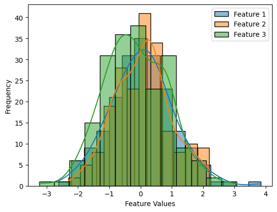
2. Data visualization
Features histogram
sns.histplot(X[:, 0], kde=True, label='Feature 1')
sns.histplot(X[:, 1], kde=True, label='Feature 2')
sns.histplot(X[:, 2], kde=True, label='Feature 3')
plt.xlabel('Feature Values')
plt.ylabel('Frequency')
plt.legend()
plt.show()
3. Training/Test sets creation
X_train, X_test, y_train, y_test = train_test_split(X, y,
test_size=0.2, random_state=42)
4. Model implementation
Cost function
def compute_loss(X, y, w, b, m):
    y_hat = np.dot(X, w) + b
    loss = (1 / (2* m)) * np.sum((y_hat - y)**2)
    return loss
The compute gradients function
def compute_gradients(X, y, w, b, m):
    y_hat = np.dot(X, w) + b
    error = y_hat - y
    dj_dw = (1 / m) * np.sum(error * X, axis = 0)
    dj_db = (1 / m) * np.sum(error)
    return dj_dw, dj_db
The optimization function (gradient descent)
def compute_optimization(learning_rate, w, b, dj_dw, dj_db):
    w_new = w - (learning_rate * dj_dw)
    b_new = b - (learning_rate * dj_db)
    return w_new, b_new
The fit(training) function
def fit(epochs, learning_rate, X, y, w, b, debug):
    m, n = X.shape

    losses = list() #tracking purposes

    for epoch in range(epochs):

        loss = compute_loss(X, y, w, b, m)
        losses.append(loss)

        dj_dw, dj_db = compute_gradients(X, y, w, b, m)
        w_new, b_new = compute_optimization(learning_rate,
w, b, dj_dw, dj_db)

        w = w_new
        b = b_new

        # print
        if (debug and (epoch % 50) == 0):
            print(f"epoch: {epoch}, loss: {loss}")

    return w, b, losses
Training the model
epochs = 500
learning_rate = 0.01

m, n = X_train.shape

w = np.random.rand(n,1)
b = np.random.rand(1)

w, b, loss = fit(epochs, learning_rate, X_train, y_train, w, b, True)
w, b
5. Prediction and model evaluation
Prediction function
def predict(X):
    return np.dot(X, w[0]) + b
Prediction and model evaluation using R-squared
R-squared ( is a metric that ranges from 0 to 1 and is sometimes expressed as a percentage between 0% and 100%. It represents the proportion of variance in the dependent variable (target) that is explained by the regression model. In other words, it indicates how much variability in target values is captured by the model.
R-squared interpretation
The model explains no variability in the data and is essentially useless for making predictions.
The model explains all the variability in the data and makes perfect predictions. This is rare in practice and could be a sign of overfitting.
The better the model fits the data. A higher value indicates that the model can explain a greater proportion of the variability in the target values.
y_pred = predict(X_test)
score = r2_score(y_test, y_pred)
score
0.7072394118821352
Final comments
In this journey through multiple linear regression, we embarked on a hands-on exploration of the fundamental concepts, implementation from scratch using Python and NumPy, and performance evaluation using the Mean Squared Error (MSE) metric and the R-squared ( ) score. Achieving an R-squared value of 0.707 demonstrates that our model captures a substantial portion of the data's variability, indicating a meaningful relationship between our predictor variables and the target. This journey not only allowed us to gain insights into the inner workings of regression modeling but also showcased the power of building predictive models from the ground up. Armed with these skills, we're well-equipped to tackle more complex regression problems and fine-tune our models for even better performance.
References
[1] A. Géron, "Hands-On Machine Learning with Scikit-Learn, Keras, and TensorFlow," O'Reilly Media, Inc., Oct. 2022.
[2] I. Goodfellow, Y. Bengio, and A. Courville, "Deep Learning," The MIT Press.

Top comments (0)