Tidyverts による時系列予測モデリング

R を使って、基本的な時系列予測モデルの構築と予測値算出を行っていきます。本投稿では、R の時系列モデリングのライブラリ tidyverts を中心に利用します。

tidyverts とは？

tidyverts は、大きく下記の3つのライブラリから構成されます。

tsibble : 時系列データに特化たデータ型を提供

fable : 時系列予測のモデルを提供

feasts : 時系列データの統計処理や特徴量抽出の機能を提供

Microsoft Forecasting Best Practice

Microsoft が Forecasting の Best Practice 集を公開しています。

microsoft / forecasting

Time Series Forecasting Best Practices & Examples

Forecasting Best Practices

Time series forecasting is one of the most important topics in data science. Almost every business needs to predict the future in order to make better decisions and allocate resources more effectively.

This repository provides examples and best practice guidelines for building forecasting solutions. The goal of this repository is to build a comprehensive set of tools and examples that leverage recent advances in forecasting algorithms to build solutions and operationalize them. Rather than creating implementations from scratch, we draw from existing state-of-the-art libraries and build additional utilities around processing and featurizing the data, optimizing and evaluating models, and scaling up to the cloud.

The examples and best practices are provided as Python Jupyter notebooks and R markdown files and a library of utility functions. We hope that these examples and utilities can significantly reduce the “time to market” by simplifying the experience from defining the…

View on GitHub

このリポジトリでも Tidyverts が利用されていますので、是非ご確認ください。

需要予測などのテーマでは、例えば "店舗" ✖️ "ブランド" ごとにモデルを作る必要があったりします。そのために並列処理の実装が欠かせません。本投稿では言及しませんが、このリポジトリでは、Python では Ray 、R では {parallel} を利用して並列処理を実装しています。

利用するデータ

Prophet のチュートリアルで使用されている Peyton Manning の Wikipedia の閲覧者数の時系列データを利用します。下記 URL から CSV データをダウンロードしておきます。

example_wp_log_peyton_manning.csv

分析環境

R Studio や Visual Studio Code で構いません。私は Azure Machine Learning で提供している PaaS の R Studio を利用しています。

Azure Machine Learning

R Support in Azure Machine Learning | AI Show | Channel9

ライブラリのロード

利用するライブラリをロードします。

library(fable)
library(fable.prophet)
library(tsibble)
library(tsibbledata)
library(feasts)
library(lubridate)
library(dplyr)
library(ggplot2)

データ準備と探索

CSV ファイルのパスを指定して、データをロードします。

df <- read.csv("example_wp_log_peyton_manning.csv", colClasses=c("Date","numeric")) 

df に格納されているデータを tsibble形式に変換し可視化します。"%>%" は R 言語で利用されるパイプ処理を意味しています。autoplot を適用すると可視化まで簡単にできます。

df %>% as_tsibble %>% autoplot

df %>% as_tsibble %>% fill_gaps

fill_gaps を利用して、データに欠損している日時項目を補完します。また tidyr の fill で欠損値を補完します。１つ先の時系列データ値を用いて補完する場合は、.direction = down と指定します。

df_filled <- df %>% as_tsibble %>% fill_gaps %>% tidyr::fill(y, .direction = "down")

次に feasts ライブラリの STL を用いて、時系列データを "季節" "トレンド" "不規則成分" に分解します。

dcmp <- df_filled %>%
    model(STL(y ~ season(window = Inf ))) %>% components
dcmp

可視化して特徴を確認します。Weekly の季節性トレンドは細かすぎて黒塗りに見えちゃっているようです。

dcmp %>% autoplot

時系列モデルの構築と予測値算出

まずは非常にシンプルなモデルを試します。データには季節性などが確認されるものの、これらのモデルは考慮してくれないことが分かります。

• MEAN : 平均値
• NAIVE(=RW): ランダムウォークモデル

ここでは、ドリフトを考慮するモデルも追加します。このデータは後半にトレンドが減少している傾向にあるので、このモデルも減少方向に予測していることが確認できます。

df_filled %>% 
    model(
        mean=MEAN(y),
        naive=NAIVE(y),
        drift=RW(y ~ drift()),  # ドリフトを考慮
        .safely=FALSE) %>% 
    forecast(h="2 years") %>% 
    autoplot(filter(as_tsibble(df_filled),year(ds) > 2007), level = NULL)

次に季節性を考慮します。

• SNAIVE : 季節性を考慮するランダムウォークモデル

1年周期の季節性があるデータなので、過去 1 年前のデータを予測とするモデルを採用します。

df_filled %>% 
    model(
        mean=MEAN(y),
        naive=NAIVE(y),
        drift=RW(y ~ drift()),  # ドリフトを考慮
        snaive = SNAIVE(y ~ lag("year")), # 季節性を考慮
        .safely=FALSE) %>% 
    forecast(h="2 years") %>% 
    autoplot(filter(as_tsibble(df_filled),year(ds) > 2007), level = NULL)

次に指数平滑化を使用します。

• ETS : 指数平滑化

1年周期を適用してみます。

df_filled %>% 
    model(
        est=ETS(y ~ season("A", period= "1 year")),
        .safely=FALSE) %>% 
    forecast(h="1 year") %>% 
    autoplot(filter(as_tsibble(df_filled),year(ds) > 2015), level = NULL)

すると、エラーが出てきました。

Error: Seasonal periods (period) of length greather than 24 are not supported by ETS.

最大 24 サイクルしか考慮してくれないようです。このデータは Daily のデータなので、年周期の季節性の考慮は難しそうです。

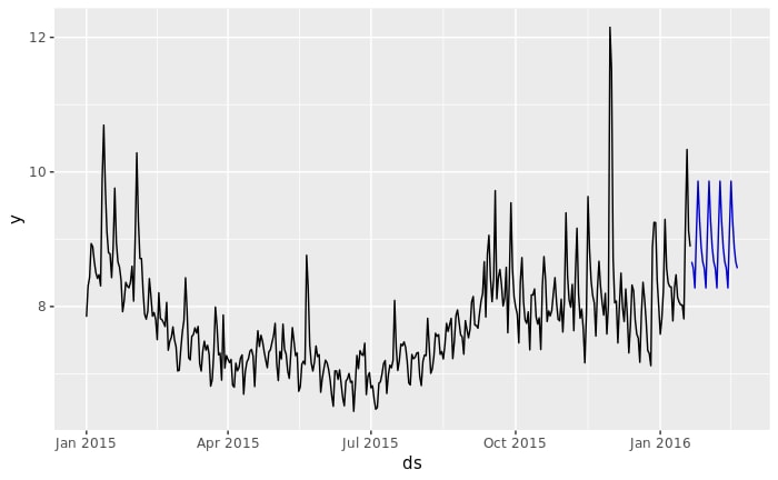
週周期の季節性があると想定して、モデル構築と予測値算出を行います。

df_filled %>% 
    model(
        est=ETS(y ~ season("A", period= "7 days")),
        .safely=FALSE) %>% 
    forecast(h="30 days") %>% 
    autoplot(filter(as_tsibble(df_filled),year(ds) > 2014), level = NULL)

次に ARIMA モデルを利用します。ETS ではうまく動きませんでしたが、ARIMA では、period や D=1 を設定することで年周期の季節性も考慮してくれます。

• (S)ARIMA : (季節)自己回帰和分移動平均

df_filled %>% 
    model(
        arima=ARIMA(y ~ pdq(1,1,3) + PDQ(0,1,0,period="365 days")),
        .safely=FALSE) %>%
        forecast(h="2 years") %>% 
    autoplot(filter(as_tsibble(df_filled),year(ds) > 2007), level = NULL)

次に、Facebook の Prophet を利用します。fable.prophet というライブラリが公開されており、いままで使ってきた fable でも Prophet のモデルを組み込めるようになっています。詳細は fable.prophet からご確認ください。

df_filled %>% 
    model(
        prophet(y),
        .safely=FALSE) %>% 
    forecast(h="2 years") %>% 
    autoplot(filter(as_tsibble(df_filled),year(ds) > 2007), level = NULL)

以上です。