
The source code for the topics discussed in the post can be found at https://github.com/ML-Scratch/ML_Code_From_Scratch
Linear regression is a very basic supervised learning model. It is used when there is a linear relationship between the feature vector and the target , or in simple terms between the input and output we are trying to predict. Linear regression serves as the starting point for many machine learning enthusiasts and understanding this model can greatly help in mastering the more complex models in ML.
When should you use Linear Regression?
As the name suggests, Linear Regression involves fitting the best fit straight line through the data. Consider a dataset consisting information of used cars and the prices they were sold for. For example, it consists of the number of kilometers the car traveled and the price it was sold. As one might realize, there could be a linear relationship between the number of kilometers traveled and the selling price.
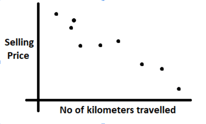
A visualisation of the data like in the above image makes it clear that a straight line can be fit for this kind of data. One should also note that in most of the cases it is impossible to fit at line that passes through all the points in the dataset. The best we could do is to fit a straight line that looks like passing through most of the points and we will see in the coming sections how we could do so. Once we fit a line through this data i.e generate a line equation, we can start predicting prices by plugging in the number of kilometers the car has traveled into the line equation.
Understanding the math
The math behind the working of Linear regression is not at all complicated. For simplicity let’s assume we have only one feature i.e the no kilometers traveled (let's call this X) in the dataset and one column with the selling prices of these cars (let's call this Y).
Our job is to create a line equation like Y = mX + c . When the value of X (i.e the number of kilometers traveled) from the dataset is plugged into this equation it should calculate Y (i.e the predicted selling price) that is either equal to the selling price value from the dataset or some close enough value.
As you might incur, the variables in the above line equation are m and c which are nothing but the slope of the line and the y intercept of the line. Remember that X and Y are not the variables in our case as they are nothing but constants from our dataset that we will use in creating the best fit line.
So our job is now to find out the right m and c values so that we can make an ideal straight line that passes through most of the points in the dataset.
Let's modify the above equation slightly to Y = θ0 + θ1X
Where θ0 = c and Y = θ1 = m.
How to decide if a line is good enough?
Now that we understand the line equation, how should we decide if the line equation we are using the best fit line or not. An obvious way to do this is to plot the line against the dataset and visually decide.

However this is not practically possible for huge datasets with large no of features, which is often the case with most of the real world datasets. Hence we use a simple mathematical formula called the cost function to decide if a given line is a good fit or a bad fit to the data.
Consider the following mini dataset:
| S.no | Km's travel | Price |
|---|---|---|
| 1 | 1000 | 2.1 |
| 2 | 2000 | 1.7 |
Suppose we start with random values for θ0 = 10 and θ1 = 20. Let us plug in X = 1000 as per the first example in the dataset.
Y = 10 + 20(1000)Y = 20010
The predicted value according to the above equation is 20010 rupees whereas the selling price according to the dataset is 200000 rupees. This is definitely a bad prediction. The magnitude of the badness of this prediction or technically the error is the difference in the predicted value(denoted by Ŷ and the actual value(denoted by Y).
In this the predicted value Ŷ = 20010 where as the actual value(or value from the dataset) is Y = 210000.
The cost function for two variables θ0 and θ1 are denoted by J and is given as follows

The cost function calculates the square of the error for each example in the dataset, sums it up and divides this value by the number of examples in the dataset (denoted by m).
This cost function helps in determining the best fit line.
Note: The division with 2 is to simplify calculations involving the first order differentials
Arriving at the best fit line
Now that we have defined the cost function, we have to make use of it to adjust our parameters θ0 and θ1 such that they result in the least cost function value. We make use of a technique called Gradient Descent to minimize the value of the cost function.
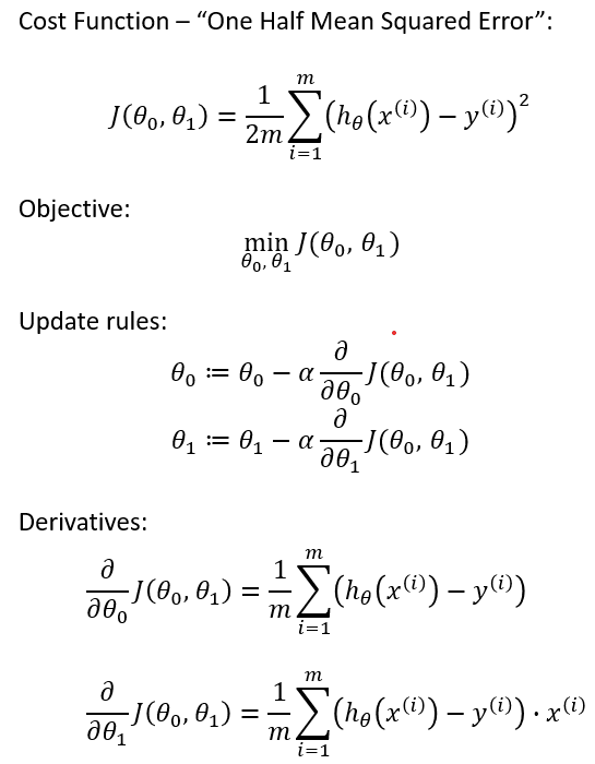
Gradient descent makes small changes to existing θ0 and θ1 values such that they result in more and more smaller cost function values. The changes to θ0 and θ1 are performed as follows.

Where j = 0 or j = 1
Let's try to understand, what this updating to θ0 and θ1 mean?
The differential part of this equation i.e determines whether we have to increment or decrement the value θj. If this differential is a positive value then θj is decremented and if this differential is a negative value then θj is decremented as it can be observed from the above equation.
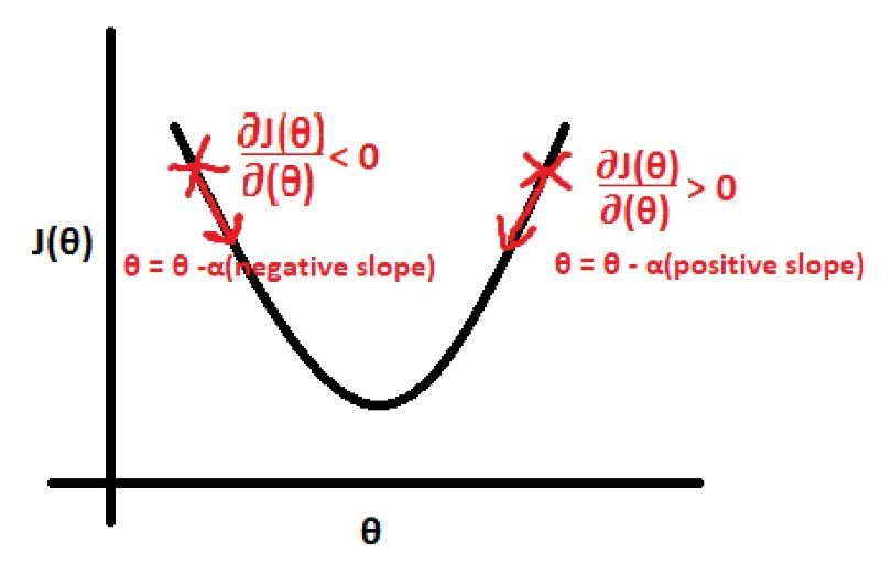
Now that we know if we have to increment or decrement θj, next we have to determine by how much θj should be changed. This is what α or the learning rate indicates. Larger the α value, the larger is the updation for θj and vice versa. The value of α should not be too small as it will result in very slow convergence to the best fit line and it should not be too large as we might miss the values of θj which result in the best fit line.
One set of updations of θj is called an iteration of Gradient Descent.
This process of updation is repeated till the point where the cost function value remains largely unchanged.

After a sufficient number of iterations of gradient descent, we can visually check the performance the line by plotting it against the values in the dataset. If everything goes right, you should have a pretty decent line. You can now use this line equation to make predictions for any given X value (or the number of kilometers traveled).
Pros
- Space complexity is very low it just needs to save the weights at the end of training. Hence it's a high latency algorithm
- Its very simple to understand
- Good interpretability
- Feature importance is generated at the time model building
- With the help of hyperparameter lambda, you can handle features selection hence we can achieve dimensionality reduction
- Small number of hyperparmeters
- Can be regularized to avoid overfitting and this is intuitive
- Lasso regression can provide feature importances
Cons
- The algorithm assumes data is normally distributed in real but they are not
- Before building a model multi-collinearity should be avoided.
- Prone to outliers.
- Input data need to be scaled and there are a range of ways to do this.
- May not work well when the hypothesis function is non-linear.
- A complex hypothesis function is really difficult to fit. This can be done by using quadratic and higher order features, but the number of these grows rapidly with the number of original features and may become very computationally expensive.
- Prone to overfitting with a large number of features are present.
- May not handle irrelevant features
So far so good, we have learned overview of Linear Regression our next post revolves around the math concepts involved in Linear Regression.
Read On 📝
Contributors
This series is made possible by help from:
- Pranav (@devarakondapranav )
- Ram (@r0mflip )
- Devika (@devikamadupu1 )
- Pratyusha(@prathyushakallepu )
- Pranay (@pranay9866 )
- Subhasri (@subhasrir )
- Laxman (@lmn )
- Vaishnavi(@vaishnavipulluri )
- Suraj (@suraj47 )

Top comments (2)
I like your explanation of linear regression. I want to know if you write articles on other topics of machine learning or not.
I also like to share my blog link so anyone can view it and provide me with their thoughts: -linear regression