
Maximum Likelihood Estimation , or MLE, for short, is the process of estimating the parameters of a distribution that maximize the likelihood of the observed data belonging to that distribution.
Simply put, when we perform MLE, we are trying to find the distribution that best fits our data. The resulting value of the distribution’s parameter is called the maximum likelihood estimate.
MLE is a very prominent frequentist technique. Many conventional machine learning algorithms work with the principles of MLE. For example, the best-fit line in linear regression calculated using least squares is identical to the result of MLE.
The likelihood function
Before we move forward, we need to understand the likelihood function.
The likelihood function helps us find the best parameters for our distribution. It can be defined as shown:

where θ is the parameter to maximize, x_1, x_2, … x_n are observations for n random variables from a distribution and f is the joint density function of our distribution with the parameter θ.
The pipe (“ | “) is often replaced by a semi-colon, since θ isn’t a random variable, but an unknown parameter.
Of course, θ could also be a set of parameters.

For example, in the case of a normal distribution, we would have
θ = (μ,σ), with μ and σ representing the two parameters of our distribution.
Intuition
Likelihood is often interchangeably used with probability, but they are not the same. Likelihood is not a probability density function, meaning that integrating over a specific interval would not result in a “probability” over that interval. Rather, it talks about how likely a distribution with certain values for its parameters fits our data.

Looking at it this way, we can say that likelihood is how likely the distribution fits of given data for variable values of its parameters. So, if L(θ_1|x) is greater than L(θ_2|x), the distribution with parameter value as θ_1 fits our data better than the one with a parameter value of θ_2.
Process
To re-iterate, we’re looking for the parameter (or parameters, as the case may be) that maximize our likelihood function. How do we do that?
To simplify our calculations, lets assume that our data is independently and identically distributed , or i.i.d, for short, meaning that observations are independent of each other and that they can be quantified in the same way, which basically means that all points are from the same distribution.
The i.i.d assumption allows us to easily calculate the cumulative likelihood considering all data points as a product of individual likelihoods.
Also, most likelihood functions have a single maxima, allowing us to simply equate the derivate to 0 to get the value of our parameter. If multiple maxima exist, we would need to look at the global maxima to get our answer.
In general, more complex numerical methods would be required to find the maximum likelihood estimate.
An Example
To understand the math behind MLE, let’s try a simple example. We’ll derive the value of the exponential distribution ’s parameter corresponding to the maximum likelihood value.
The Exponential Distribution
The exponential distribution is a continuous probability distribution used to measure inter-event time.
It has a single parameter, called λ by convention. λ is called rate.
Its mean and variance is 1/ λ and 1 / λ², respectively.
The probability density function for the exponential distribution is as shown below.


There’s a single parameter λ. Let’s calculate its value, given n random points x_1 to x_n.
As discussed earlier, we know that the likelihood for a given point xi is given by the following:

We calculate the likelihood for each of our n points.

The combined likelihood for all n points would just be the product of their individual likelihoods, since we are considering independent and identically distributed points.

The log-likelihood
Our next step would be to find the derivative of our likelihood function and set it to 0, since we want to find the value of our distribution parameter (in this case, λ) which gives the maximum likelihood.
Since the derivatives of both functions and those of their logarithms have the same stationary points (derivative equates to 0), we can simplify our calculations by considering the logarithm of our likelihood function.
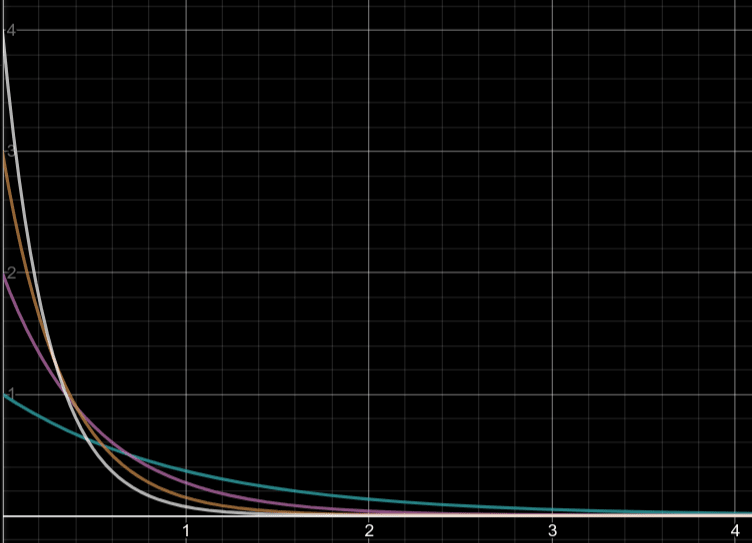
Lets plot a simple graph that represents the following equations when a and b are both set to 1. The rate parameter, λ, has been replaced by x.

The terms a and b represent two datapoints, say, x_1 and x_2. Our likelihood function is represented by the orange curve. It is the product of likelihoods of the two individual datapoints.
The logarithm of the likelihood function, or the log-likelihood , is represented by the pink curve.

The blue-dotted line will be covered later.
Two things to notice:
- Both the likelihood function (orange) and its logarithm (pink) have the same stationary point (the derivative is 0).
- That common stationary point occurs at the x=1 (blue curve), which may not make much sense at the moment, is basically a simple proof of our result. We’ll revisit this point after obtaining our result.

The product of small probabilities, as is the case in calculating the likelihood over several data points, can also lead to numerical underflow due to very small probabilities, giving us another reason to prefer working with the “sum of logs” rather than “products”.

Simplifying our result, we get:

This is the log-likelihood for the exponential distribution.
The derivative
Now that we have our log-likelihood function, lets find its maxima. To do this, we simply find its first derivative with respect to λ.
Differentiating log (L(λ)), we get:

Following that, we end up with:

Simplying this further, we get the following relation for λ:

So the value of λ that maximizes likelihood can be calculated using the above relation. Similar calculations can be done for other continuous and even discrete distributions.
Now, coming back to our graph example, the blue dotted line, with the equation: x = 2 / (a + b), is our value for λ when n is 2.
Remember, the value of λ we obtained represents the maximum value of likelihood function (orange curve). For a = 1 and b = 1, we get x = 1 and hence λ = 1, which is shown in the graph as the maxima of the orange curve.
In distributions with multiple parameters, like the normal distribution, we consider each one in turn, keeping the others constant.
Conclusion
MLE isn’t the only technique which helps us do this. Other techniques include
- Maximum A Priori Estimation (MAP), which uses prior data as well, unlike MLE, which considers a uniform prior; and
- Expectation Maximization, which handles latent variables (those unobservable variables which have an effect on present variables), something that MLE struggles with.
There’s a lot more to Maximum Likelihood Estimation — and for that matter, other parameter estimation techniques. This post focuses more on the underlying math behind MLE using the exponential distribution as an example.
Hopefully, this article gets you started with other, more complex techniques!
Of course, please let me know in the comments if anything’s unclear and I’ll update the post. Thanks for reading!

Top comments (0)