
TLDR;
Colab Notebook
In agriculture, leaf diseases cause a major decrease in both quality and quantity of yields. Automating plant disease detection using Computer Vision could play a role in early detection and prevention of diseases.
What will you build!

In this exercise we will explore how to build a plant leaf disease classifier using Monk’s quick Hyper-Parameter finding feature.
Monk provides a syntax invariant transfer learning framework that supports Keras, Pytorch and Mxnet in the backend. (Read — Documentation).
Computer Vision developers have to explore strategies while selecting the correct learning rates, a fitting CNN architecture, use the right optimisers and fine-tune many more parameters to get the best performing models.
The Hyper-Parameter finding features assists in analysing multiple options for a selected hyper-parameter before proceeding with the actual experiment. This not just saves a lot of time spent in prototyping but also assists in quickly exploring the how well a selected set of parameters perform on the dataset in use and the final application.
Let’s begin!
Setup
We start by setting up Monk and it’s dependencies on colab. For further setup instructions on different platforms check out the DOCS.
$ git clone https://github.com/Tessellate-Imaging/monk_v1
$ cd monk_v1/installation && pip install -r requirements_cu10.txt
$ cd ../..
Dataset
For this exercise we will use dataset gathered by the awesome folks at PlantVillage.
Experimentation
Before setting up our analysis, we have to start by creating a new project and experiment
# Step 1 - Create experimentptf = prototype(verbose=1);ptf.Prototype("plant_disease", "exp1");
and setup the ‘Default’ dataset paths
ptf.Default(dataset_path=["./dataset/train", "./dataset/val"],
            model_name="resnet18",
            freeze_base_network=True, num_epochs=5);
Now we are ready to run some analysis and find the best Hyper-Parameters.
Currently we can analyse the following parameters :
- Find the best CNN architecture — DOCS
- Find the right batch size — DOCS
- Find the a good input shape — DOCS
- Select a good starting learning rate — DOCS
- Select the best performing Optimiser — DOCS
We will analyse each of the above parameters to select the best and finally train our model to build the application of Plant Leaf disease classification.
Model Finder
Start by giving a name to the analysis. For every analysis a new project is created with multiple experiments inside.
analysis_name = “Model_Finder”;
Now we pass on the list of Models from which to analyse
- First element in the list — Model Name
- Second element in the list — Boolean value to freeze base network or not
- Third element in the list — Boolean value to use pretrained model as the starting point or not
models = [[“resnet34”, True, True], [“resnet50”, False, True],[“densenet121”, False, True], [“densenet169”, True, True], [“densenet201”, True, True]];
Set the Number of epochs for each experiment to run
epochs=5;
Select the Percentage of original dataset to take in for experimentation
percent_data=10;
Finally we run the analysis function to search for best performing models:
- “keep_all” — Keeps all the experiments created
- “keep_none” — Deletes all experiments created
ptf.Analyse_Models(analysis_name, models,
                   percent_data, num_epochs=epochs,
                   state=”keep_none”);
When the analysis is running, the estimated time is displayed for every experiment
Running Model analysis
Analysis Name : Model_Finder Running experiment : 1/5
Experiment name : Model_resnet34_freeze_base_pretrained
Estimated time : 2 min
Finally after the experiment is completed we receive the following output on training and validation accuracies and losses:
 Experiment Output
Select the best performing CNN architecture, update your experiment and continue with further analysis. Don’t forget to reload the experiment after updating.
## Update Model Architecture
ptf.update_model_name(“densenet121”);
ptf.update_freeze_base_network(False);
ptf.update_use_pretrained(True);
ptf.Reload();
For further instructions on updating experiment parameters, check out the documentation.
Batch Size Finder
# Analysis Project Name
analysis_name = “Batch_Size_Finder”;# Batch sizes to explore
batch_sizes = [4, 8, 16, 32];# Num epochs for each experiment to run
epochs = 10;# Percentage of original dataset to take in for experimentation
percent_data = 10;
ptf.Analyse_Batch_Sizes(analysis_name, batch_sizes,
                        percent_data,
                        num_epochs=epochs, state=”keep_none”);
Generated output:
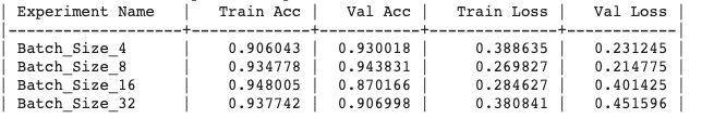 Experiment Output
Update the experiment :
## Update Batch Size
ptf.update_batch_size(8);
ptf.Reload();
Input Shape Finder
# Analysis Project Name
analysis_name = “Input_Size_Finder”;# Input sizes to explore
input_sizes = [224, 256, 512];# Num epochs for each experiment to run
epochs=5;# Percentage of original dataset to take in for experimentation
percent_data=10;
ptf.Analyse_Input_Sizes(analysis_name,
                        input_sizes, percent_data,
                        num_epochs=epochs, state=”keep_none”);
Generated output :
 Experiment Output
Update the experiment :
## Update Input Sizeptf.update_input_size(224);
ptf.Reload();
Learning Rate Analysis
# Analysis Project Name
analysis_name = “Learning_Rate_Finder”# Learning rates to explore
lrs = [0.01, 0.005, 0.001, 0.0001];# Num epochs for each experiment to run
epochs=5# Percentage of original dataset to take in for experimentation
percent_data=10
ptf.Analyse_Learning_Rates(analysis_name, lrs, percent_data,
                           num_epochs=epochs, state=”keep_none”);
Generated output :
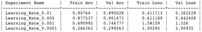 Experiment Output
Update the experiment :
## Update Learning Rateptf.update_learning_rate(0.01);
ptf.Reload();
Optimiser Analysis
# Analysis Project Name
analysis_name = “Optimiser_Finder”;# Optimizers to explore
optimizers = [“sgd”, “adam”, “adamax”, “rmsprop”]; #Model name
epochs = 5;# Percentage of original dataset to take in for experimentation
percent_data = 10;
ptf.Analyse_Optimizers(analysis_name, optimizers, percent_data,
                       num_epochs=epochs, state=”keep_none”);
Generated output :
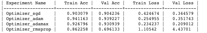 Experiment Output
Update the experiment :
## Update Optimiserptf.optimizer_adamax(0.001);
ptf.Reload();
Training
Finally after setting the correct hyper-parameters, we can begin training the model.
ptf.Train();
Copy Experiment
We can visualise the accuracy and loss plots, located inside the workspace directory. From the plots we observe that the losses can go further down:
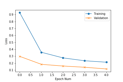 Loss curves
To continue training, we copy our previous experiment and resume from that state — DOCS
Compare Experiments
After finishing our training we can compare both these experiments to check if we actually improved performance using Compare Experiment feature in Monk.
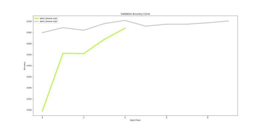 Validation accuracy curves
Our ‘experiment 1’ ran for 5 epochs and ‘experiment 2’ ran for 10 epochs. Even though a minor improvement in validation accuracy, an increase from 96% to 97% could help achieve leader board positions for competitions hosted on Kaggle and EvalAi.
Hope you have fun building niche solutions with our tools.
Happy Coding!

Top comments (0)