PRINCIPAL COMPONENT ANALYSIS - WITH HANDS ON MINI PROJECT !!

Principal Component Analysis is an unsupervised statistical technique used to examine interrelations among a set of variables in order to identify the underlying structure of those variables.
It is a linear dimensionality reduction technique that can be utilized for extracting information from a high-dimensional space by projecting it into a lower-dimensional sub-space. It tries to preserve the essential parts that have more variation of the data and remove the non-essential parts with fewer variation

It is sometimes also known as general factor analysis.

As Regression which I have explained in previous article determines a line of best fit to a data set , factor analysis determines several orthogonal lines of best fit to the data set.

Orthogonal means at "right angles" i.e the lines are perpendicular to each other in any 'n' dimensional space.

Here we have some data plotted along two features x and y

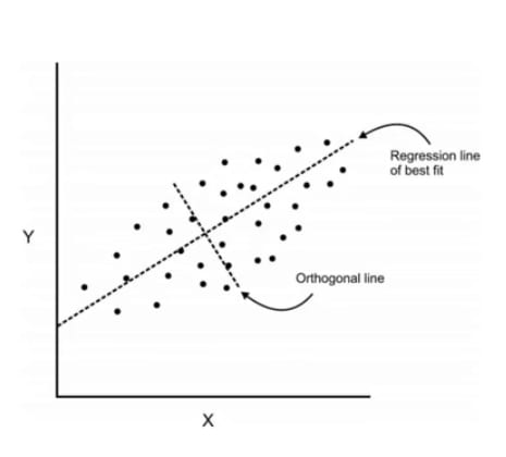
We can add an orthogonal line. Components are a linear transformation that chooses a variable system for a data set such that the greatest variance of the data set comes to lie on the first axis

The second greatest variance on the second axis and so on ...
This process allows us to reduce the number of variables used in an analysis.
Also keep in mind that the components are uncorrelated , since in the sample space they are orthogonal to each other.

We can continue this analysis into higher dimensions

WHERE CAN WE APPLY PCA ???

Data Visualization: When working on any data related problem, the challenge in today's world is the sheer volume of data, and the variables/features that define that data. To solve a problem where data is the key, you need extensive data exploration like finding out how the variables are correlated or understanding the distribution of a few variables. Considering that there are a large number of variables or dimensions along which the data is distributed, visualization can be a challenge and almost impossible.
Hence, PCA can do that for you since it projects the data into a lower dimension, thereby allowing you to visualize the data in a 2D or 3D space with a naked eye.

Speeding Machine Learning (ML) Algorithm: Since PCA's main idea is dimensionality reduction, you can leverage that to speed up your machine learning algorithm's training and testing time considering your data has a lot of features, and the ML algorithm's learning is too slow.

Let us walk through the cancer data set and apply PCA

Breast Cancer
The Breast Cancer data set is a real-valued multivariate data that consists of two classes, where each class signifies whether a patient has breast cancer or not. The two categories are: malignant and benign.

The malignant class has 212 samples, whereas the benign class has 357 samples.

It has 30 features shared across all classes: radius, texture, perimeter, area, smoothness, fractal dimension, etc.

You can download the breast cancer dataset from
here
, or rather an easy way is by loading it with the help of the sklearn library.

import matplotlib.pyplot as plt
import pandas as pd
import numpy as np
import seaborn as sns
%matplotlib inline

from sklearn.datasets import load_breast_cancer
cancer = load_breast_cancer()
cancer.keys()

df = pd.DataFrame(cancer['data'],columns=cancer['feature_names'])
#(['DESCR', 'data', 'feature_names', 'target_names', 'target'])

PCA Visualization
As we've noticed before it is difficult to visualize high dimensional data, we can use PCA to find the first two principal components, and visualize the data in this new, two-dimensional space, with a single scatter-plot. Before we do this though, we'll need to scale our data so that each feature has a single unit variance.

from sklearn.preprocessing import StandardScaler

scaler = StandardScaler()
scaler.fit(df)

scaled_data = scaler.transform(df)

PCA with Scikit Learn uses a very similar process to other preprocessing functions that come with SciKit Learn. We instantiate a PCA object, find the principal components using the fit method, then apply the rotation and dimensionality reduction by calling transform().

We can also specify how many components we want to keep when creating the PCA object.

from sklearn.decomposition import PCA

pca = PCA(n_components=2)
pca.fit(scaled_data)

Now we can transform this data to its first 2 principal components.

x_pca = pca.transform(scaled_data)

scaled_data.shape
x_pca.shape

Great! We've reduced 30 dimensions to just 2! Let's plot these two dimensions out!

plt.figure(figsize=(8,6))
plt.scatter(x_pca[:,0],x_pca[:,1],c=cancer['target'],cmap='plasma')
plt.xlabel('First principal component')
plt.ylabel('Second Principal Component')

Clearly by using these two components we can easily separate these two classes.

This was just a small sneak peek into what PCA is . I hope you got an idea as how it works .
Feel free to respond below for any doubts and clarifications !!
I will soon be publishing this article on Geeksforgeeks