Essential Deep Learning Concepts Explained Intuitively
Are you new to deep learning and looking for a comprehensive guide to help you understand the basics and beyond? Look no further! In this article, we will delve into 20 essential deep learning concepts, starting with the basics and gradually moving on to more advanced topics. From Artificial Neural Network (ANN) to Gradient Descent and Activation Functions (Sigmoid, ReLU, SoftMax), we will explore everything you need to know to gain a solid foundation in deep learning. So, grab your coffee and let’s get started!
Neurons:
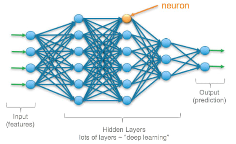
A neuron is a basic building block of a neural network. It’s like a tiny computer that can perform simple calculations and make decisions based on inputs. Neurons are connected to each other in a network, and they work together to perform complex tasks, such as image classification or language translation. The inputs to a neuron are numbers that represent the information, and the output of a neuron is a decision about what to do with that information.
Example : Let’s say you have a group of friends, and you want to play a game of “Telephone”. In this game, one person whispers a message to the next person, and so on, until the message has been passed to everyone in the group. Each person in the group is like a neuron in a neural network, receiving information from one person and passing it.
Activation Function (Sigmoid, ReLU, SoftMax)

The activation function is like a gatekeeper for each neuron in the ANN. It decides whether a neuron should be “turned on” or “turned off.” Different types of activation functions perform this decision-making process in different ways.
Sigmoid:
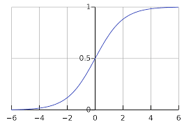
The sigmoid function is like a light switch. It turns the neuron on or off based on the input. If the input is above a certain threshold, the sigmoid function outputs a value of 1, which turns the neuron on. If the input is below the threshold, the sigmoid function outputs a value of 0, which turns the neuron off.
ReLU:

The ReLU (rectified linear unit) function is like a light switch, too, but it’s a bit more sophisticated. If the input is positive, the ReLU function outputs the same positive value, which turns the neuron on. If the input is negative, the ReLU function outputs 0, which turns the neuron off.
SoftMax:
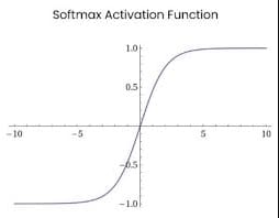
The SoftMax function is like a voting system. It takes in the outputs of all the neurons in a layer and decides which neuron should have the most influence on the final output. It does this by converting the outputs into probabilities, with the highest probability representing the most influence.
Loss Function
The loss function is like a scorecard for your ANN. It tells you how well your ANN is doing in solving the problem. Imagine you are playing a game where the goal is to get as many points as possible. The score you get after each round is the loss function. The lower the score, the better the performance of your ANN.
We have different types of Loss Function and some of them are mentioned here:
- Mean Squared Error(MSE)
- Root Mean Squared Error(RMSE)
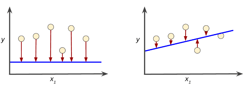
Mean Squared Error (MSE):
Mean Squared Error (MSE) is the average of the squared differences between the actual output values and the predicted values. It measures the average magnitude of the error in the predictions.
Mathematically, it is defined as:
MSE = 1/N * Σ(actual — predicted)²,
where N is the number of samples and actual and predicted are the actual and predicted values, respectively.
For example, let’s say you have a model that predicts the height of a person based on their age. You have 5 people, and their actual heights and ages are as follows:
P1 : Age = 25, Height = 170 cm
P2: Age = 28, Height = 165 cm
P3: Age = 30, Height = 160 cm
P4: Age = 32, Height = 155 cm
P5: Age = 35, Height = 150 cm
Now, let’s say your model predicts the following heights for these people:
P1: Age = 25, Height = 165 cm
P2: Age = 28, Height = 170 cm
P3: Age = 30, Height = 162 cm
P4: Age = 32, Height = 157 cm
P5: Age = 35, Height = 153 cm
The MSE of your model can be calculated as follows:
MSE = 1/5 * ( (170–165)² + (165–170)² + (160–162)² + (155–157)² + (150–153)² ) = (⁵² + ⁵² + ²² + ²² + ³²)/5 = 51
So, the MSE of your model is 51, which means the average magnitude of the error in the predictions is 51 cm².
Root Mean Squared Error (RMSE):
Root Mean Squared Error (RMSE) is the square root of the MSE. It gives the error in the same units as the actual and predicted values.
Mathematically, it is defined as:
RMSE = √(MSE)
Using the same example, the RMSE of your model can be calculated as follows:
RMSE = √(51) = 7.14 cm
So, the RMSE of your model is 7.14 cm, which means the average magnitude of the error in the predictions is 7.14 cm.
Tensor:
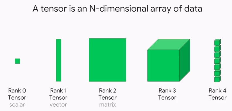
A tensor is a mathematical object that represents data. It’s like a multi-dimensional array, but more general. Think of it like a cube made of smaller cubes. The smaller cubes are like individual pieces of data, and the bigger cube is like the tensor that holds all of them together. Tensors are used in many areas of machine learning, but especially in deep learning, where they are used to store and manipulate large amounts of data.
Example: Let’s say you have data about height and weight of 10 people. You can represent this data as a 2-dimensional tensor, where each row represents the height and weight of a single person.
Artificial Neural Network (ANN):
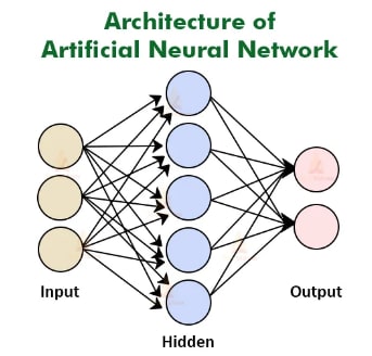
Artificial Neural Network (ANN) is a mathematical model that is inspired by the structure and function of the human brain. ANN consists of interconnected nodes, also known as artificial neurons, that process information. Each neuron receives inputs, performs a mathematical operation, and generates an output.
Example: Imagine you’re trying to identify whether a fruit is an apple or an orange based on its color and shape. You might start by asking a few questions: “Is the fruit round?” and “Is the fruit red?” Based on the answers to these questions, you would be able to determine whether the fruit is an apple or an orange.
Forward Propagation:
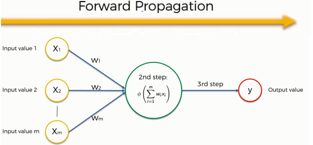
Forward Propagation is a process in deep learning where input data is passed through the neural network layers to generate the output. The input is multiplied with the weights of each layer, and the result is passed through the activation function to produce the output. This output becomes the input for the next layer until the final layer produces the final output.
Example: Imagine you have a math problem where you have to find the answer by solving multiple steps. Forward propagation is like solving those steps one by one and passing the results to the next step. This continues until the final step where we get the answer.
In the same way, in a neural network, forward propagation is the process of passing input data through the network, layer by layer, until the final output is generated. At each layer, the data is transformed based on the weights and biases of the neurons present in that layer.
Backpropagation
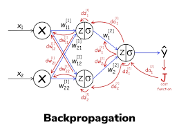
Backpropagation is an algorithm used to train artificial neural networks (ANNs). It is a supervised learning method that involves the calculation of the gradient of the loss function with respect to the network weights. The goal of backpropagation is to update the weights in a way that reduces the value of the loss function.
Example: Think of it as a teacher helping a student learn. The teacher sets a test, the student takes it, and the teacher marks it to see if the student got the answers right or wrong. The teacher then uses this information to guide the student in how to improve for next time.
Gradient Descent
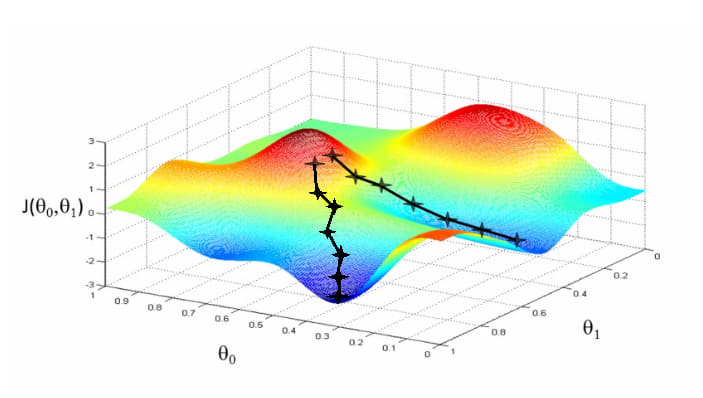
Gradient descent is one of the most popular optimizers. It’s a way to update the parameters of the model so that the loss function decreases. The idea is to calculate the gradient of the loss function with respect to the parameters and then take a step in the direction that decreases the loss function. This process is repeated many times until the loss function is as small as possible.
Example: Suppose you are standing at the top of a hill and trying to reach the bottom. You don’t want to take a straight path because it may not be the quickest or most efficient way down. Instead, you want to take small steps in the direction that will get you to the bottom of the hill the fastest. This is similar to gradient descent. It takes small steps in the direction that will reduce the loss and find the best solution.
Epoch:
An epoch in machine learning and artificial neural networks (ANNs) refers to one complete iteration through the entire training dataset. During an epoch, the model processes and uses the information from the training data to update its weights and biases, in order to better predict the outcome for the next iteration.
Example: It’s like taking a test multiple times, each time you take the test, you can learn from your mistakes and do better the next time. In the same way, after each epoch, the model should become better at recognizing patterns in the data.
Overfitting & Underfitting:
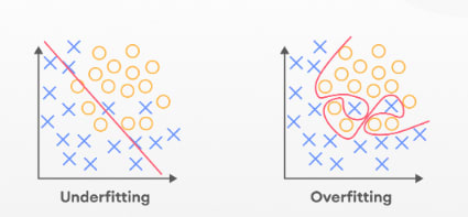
Overfitting:
Overfitting happens when a model becomes too good at recognizing patterns in the training data and becomes too specific to that data. This means that it won’t perform well on new, unseen data.
Example: Imagine a child who has memorized all the answers to a test, but doesn’t really understand the concepts. This child will perform poorly on a similar test with different questions.
Underfitting:
Underfitting is the opposite of overfitting. It occurs when a model is too simple and doesn’t have enough capacity to learn the patterns in the data.
Example: A child who doesn’t study enough for a test and doesn’t know the answers. This child will perform poorly on the test even if the questions are the same as the ones they have seen before.
Just a Quick Reminder : Feel free to follow Aspersh Upadhyay for more such interesting topics. If you want free learning resources related to Data Science and related field. Join our Telegram Channel Bit of Data Science
Cross-Validation:
Cross-validation is a technique used in machine learning to assess how well a model will perform on unseen data. The idea is to divide the data into two parts: a training set and a validation set. The model is trained on the training set and then evaluated on the validation set. This process is repeated multiple times with different parts of the data being used as the validation set each time. The goal is to see if the model is overfitting or underfitting, and to get a better idea of how it will perform on new, unseen data.
Example : Suppose you are a teacher and you have a group of 100 students and you want to test how well they know their multiplication tables. You can divide the students into two groups of 50 each. The first group of 50 students is used to train the model, while the second group of 50 students is used to validate it. You repeat this process several times, each time using a different set of 50 students for validation. This way, you get a good idea of how well the students know their multiplication tables, without having to test all 100 of them at once.
Hyperparameter Tuning:
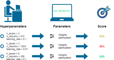
Hyperparameter tuning is the process of selecting the best set of hyperparameters for a machine learning model. Hyperparameters are parameters that are set before training a model and can’t be learned from the data. Examples of hyperparameters include the learning rate, the number of hidden layers in a neural network, or the number of trees in a random forest. The goal of hyperparameter tuning is to find the set of hyperparameters that lead to the best performance on a validation set.
Example : Let’s say you have a recipe for baking a cake. The ingredients in the recipe are like the hyperparameters of a machine learning model. You can change the ingredients in the recipe to see how it affects the taste of the cake. For example, you can try adding more sugar or less flour to see what happens. This is like hyperparameter tuning in machine learning, where you try different combinations of hyperparameters to see which one works best.
Convolutional Neural Network (CNN):
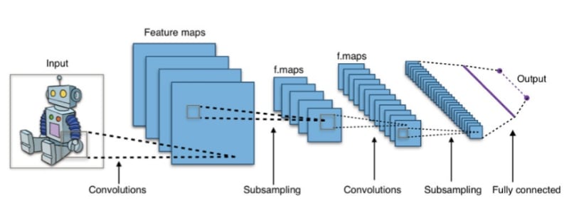
A Convolutional Neural Network is a type of artificial neural network that is especially good at analyzing images and videos. It uses a mathematical operation called convolution to scan the image and identify patterns, like shapes or edges.
Example: Think of it like a detective who is looking for clues in a picture, but instead of looking one pixel at a time, the CNN looks at multiple pixels at once to find patterns.
Batch Normalization:
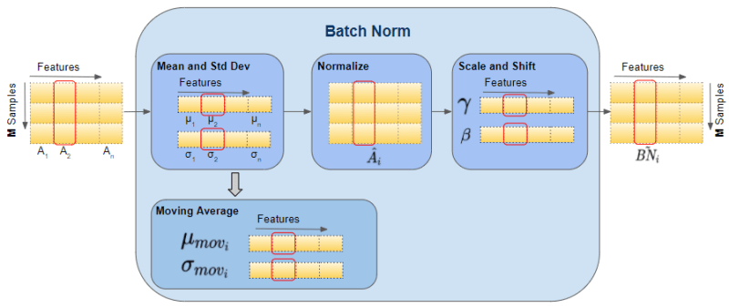
Batch normalization (BN) is a technique for improving the stability and speed of training deep neural networks. It works by normalizing the activations of neurons in a layer, which helps to make sure that they are all about the same scale. This can help to prevent the vanishing and exploding gradient problems, and it can also make the training process more efficient.
BN is typically implemented as a layer in a neural network. The layer takes the activations from the previous layer as input, and it normalizes them using the following steps:
- Calculate the mean and standard deviation of the activations.
- Subtract the mean from each activation.
- Divide each activation by the standard deviation.
- Optionally, scale and shift the activations using learnable parameters.
Scenario to use Batch Normalization:
Assume that you have a neural network with two layers. The first layer has 100 neurons, and the second layer has 10 neurons. The activations of the neurons in the first layer are all over the place. Some of them are very large, and some of them are very small. This can make it difficult for the network to learn, because the gradient of the loss function can be very large or very small, which can make it difficult for the network to find the optimal weights.
Dropout:
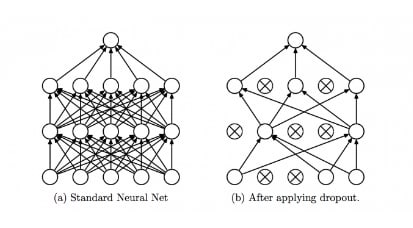
Dropout is a technique used to prevent overfitting in deep learning models. It works by randomly dropping out some of the neurons (or brain cells) during each epoch. This forces the model to learn multiple different representations of the data, which helps to prevent it from becoming too specific to the training data.
Example: Having multiple people trying to solve the same problem, each person will come up with a different solution, and by combining their solutions, you get a better result.
Recurrent Neural Network (RNN):

A Recurrent Neural Network is a type of neural network that is used for processing sequences of data. The main idea behind RNNs is to use the same weights for processing all elements in a sequence, so that the network can retain information about the sequence elements processed so far. An RNN can be used for tasks such as language translation, speech recognition, and text generation.
Long Short-Term Memory (LSTM):

Image Source: Towards AI
LSTM is a type of Recurrent Neural Network that is designed to handle the vanishing gradient problem. The vanishing gradient problem occurs when training an RNN and the gradients of the loss with respect to the weights become very small, making it difficult to update the weights effectively. LSTM solves this problem by using gates to control the flow of information and gradients through the network.
Transfer Learning:

Image source: TOPBOTS
Transfer learning is a technique in deep learning where a pre-trained neural network model is fine-tuned for a different but related task. For example, a pre-trained image classification model can be fine-tuned for object detection or segmentation. Transfer learning allows for faster training and better performance compared to training a model from scratch.
Autoencoder:
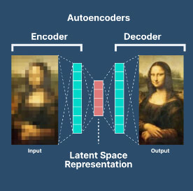
Image source: V7 Labs
An Autoencoder is a type of neural network that is used for unsupervised learning. The main idea behind Autoencoders is to learn a compact representation of the input data and then use this representation to reconstruct the input data. Autoencoders can be used for tasks such as dimensionality reduction and anomaly detection.
Generative Adversarial Network (GAN):
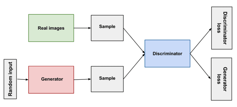
Image source: Google ML Course
A Generative Adversarial Network is a type of neural network that is used for generative modeling. The main idea behind GANs is to train two networks, a generator and a discriminator, against each other. The generator tries to generate data that looks similar to the real data, and the discriminator tries to distinguish the generated data from the real data. The goal is to find a balance between the two networks, where the generator generates data that is indistinguishable from the real data.
Conclusion:
Deep learning is a subfield of machine learning that is inspired by the structure and function of the human brain and uses artificial neural networks (ANNs). In this article, we explored 20 essential deep learning concepts starting from the basics to more advanced topics.
These concepts include Artificial Neural Network (ANN), Gradient Descent, Activation Functions (Sigmoid, ReLU, SoftMax), Backpropagation, Forward Propagation, Convolutional Neural Network (CNN), Epoch, Overfitting, Batch Normalization, Dropout, Transfer Learning, Generative Adversarial Network (GAN), Autoencoder, Reinforcement Learning, Convolutional Neural Network (CNN), Recurrent Neural Network (RNN), Long Short-Term Memory (LSTM), Generative Adversarial Network (GAN), and Transfer Learning.
By understanding these concepts, beginners can gain a comprehensive and intuitive understanding of deep learning.
Note: If you have any questions regarding the data science field so join the Bits of Data Science community and ask your question over there and we will find a solution together to resolve the issues.
Wanna Free Resources for Data Science and Machine Learning Join our Telegram Community
For more exciting insights into the world of data and machine learning, be sure to follow me on Medium, Hashnode and connect with me on LinkedIn. I publish articles regularly and would love to continue the conversation with you!
If you want to support me for writing, you can buy me a cup of coffee . Would be greatly appreciated.
Happy learning!😀

Top comments (0)