Creating Generative Art using GANs on Azure ML

This post is a part of AI April initiative, where each day of April my colleagues publish new original article related to AI, Machine Learning and Microsoft. Have a look at the Calendar to find other interesting articles that have already been published, and keep checking that page during the month.

Deep Learning can look like Magic! I get the most magical feeling when watching neural network doing something creative, for example learning to produce paintings like an artist. Technology behind this is called Generative Adversarial Networks, and in this post we will look at how to train such a network on Azure Machine Learning Service.

If you have seen my previous posts on Azure ML (about using it from VS Code and submitting experiments and hyperparameter optimization), you should know that it is quite convenient to use Azure ML for almost any training tasks. However, all examples up to now have been done using toy MNIST dataset. Today we will focus on real problem: creating artificial paintings like those:

Flowers, 2019, Art of the Artificial keragan trained on WikiArt Flowers	Queen of Chaos, 2019, keragan trained on WikiArt Portraits

Those painting are produced after training the network on paintings from WikiArt. If you want to reproduce the same results, you may need to collect the dataset yourself, for example by using WikiArt Retriever, or borrowing existing collections from WikiArt Dataset or GANGogh Project.

Place images you want to train on somewhere in dataset directory. For training on flowers, here is how some of those images might look like:

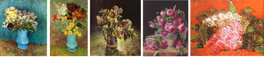
We need our neural network model to learn both high-level composition of flower bouquet and a vase, as well as low-level style of painting, with smears of paint and canvas texture.

Generative Adversarial Networks

Those painting were generated using Generative Adversarial Network, or GAN for short. In this example, we will use my simple GAN implementation in Keras called keragan, and I will show some simplified code parts from it.

shwars / keragan

Keras implementation of GANs

GAN consists of two networks:

• Generator, which generates images given some input noise vector
• Discriminator, whose role is to differentiate between real and "fake" (generated) paintings

Training the GAN involves the following steps:

1. Getting a bunch of generated and real images:

noise = np.random.normal(0, 1, (batch_size, latent_dim))
gen_imgs = generator.predict(noise)   
imgs = get_batch(batch_size)

1. Training discriminator to better differentiate between those two. Note, how we provide vector with ones and zeros as expected answer:

d_loss_r = discriminator.train_on_batch(imgs, ones)
d_loss_f = discriminator.train_on_batch(gen_imgs, zeros)
d_loss = np.add(d_loss_r , d_loss_f)*0.5

1. Training the combined model, in order to improve the generator:

g_loss = combined.train_on_batch(noise, ones)

During this step, discriminator is not trained, because its weights are explicitly frozen during creation of combined model:

discriminator = create_discriminator()
generator = create_generator()
discriminator.compile(loss='binary_crossentropy', optimizer=optimizer, 
                      metrics=['accuracy'])
discriminator.trainable = False

z = keras.models.Input(shape=(latent_dim,))
img = generator(z)
valid = discriminator(img)

combined = keras.models.Model(z, valid) 
combined.compile(loss='binary_crossentropy', optimizer=optimizer)

Discriminator Model

To differentiate between real and fake image, we use traditional Convolutional Neural Network (CNN) architecture. So, for the image of size 64x64, we will have something like this:

discriminator = Sequential()

for x in [16,32,64]: # number of filters on next layer
    discriminator.add(Conv2D(x, (3,3), strides=1, padding="same"))
    discriminator.add(AveragePooling2D())
    discriminator.addBatchNormalization(momentum=0.8))
    discriminator.add(LeakyReLU(alpha=0.2))
    discriminator.add(Dropout(0.3))

discriminator.add(Flatten())
discriminator.add(Dense(1, activation='sigmoid'))

We have 3 convolution layers, which do the following:

• Original image of shape 64x64x3 is passed over by 16 filters, resulting in a shape 32x32x16. To decrease the size, we use AveragePooling2D.
• Next step converts 32x32x16 tensor into 16x16x32
• Finally, after the next convolution layer, we end up with tensor of shape 8x8x64.

On top of this convolutional base, we put simple logistic regression classifier (AKA 1-neuron dense layer).

Generator Model

Generator model is slightly more complicated. First, imagine if we wanted to convert an image to some sort of feature vector of length latent_dim=100. We would use convolutional network model similar to the discriminator above, but final layer would be a dense layer with size 100.

Generator does the opposite - converts vector of size 100 to an image. This involves a process called deconvolution, which is essentially a reversed convolution. Together with UpSampling2D they cause the size of the tensor to increase at each layer:

generator = Sequential()
generator.add(Dense(8 * 8 * 2 * size, activation="relu", 
                                      input_dim=latent_dim))
generator.add(Reshape((8, 8, 2 * size)))

for x in [64;32;16]:
    generator.add(UpSampling2D())
    generator.add(Conv2D(x, kernel_size=(3,3),strides=1,padding="same"))
    generator.add(BatchNormalization(momentum=0.8))
    generator.add(Activation("relu"))

generator.add(Conv2D(3, kernel_size=3, padding="same"))
generator.add(Activation("tanh"))

At the last step, we end up with tensor size 64x64x3, which is exactly the size of the image that we need.
Note that final activation function is tanh, which gives an output in the range of [-1;1] - which means that we need to scale original training images to this interval. All those steps for preparing images is handled by ImageDataset class, and I will not go into detail there.

Training script for Azure ML

Now that we have all pieces for training the GAN together, we are ready to run this code on Azure ML as an experiment! The code I will be showing here is available at GitHub:

CloudAdvocacy / AzureMLStarter

This is some tutorial to get you started with Azure ML Service

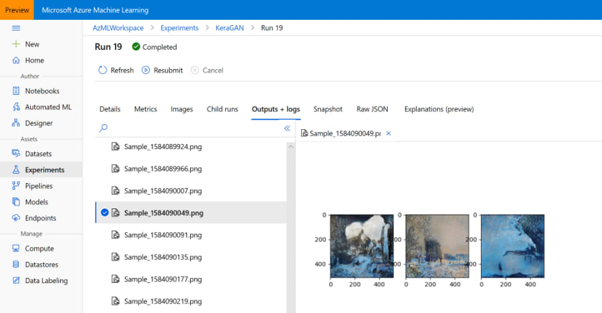
There is one important thing to be noted, however: normally, when running an experiment in Azure ML, we want to track some metrics, such as accuracy or loss. We can log those values during training using run.log, as described in my previous post, and see how this metric changes during training on Azure ML Portal.

In our case, instead of numeric metric, we are interested in the visual images that our network generates at each step. Inspecting those images while experiment is running can help us decide whether we want to end our experiment, alter parameters, or continue.

Azure ML supports logging images in addition to numbers, as described here. We can log either images represented as np-arrays, or any plots produced by matplotlib, so what we will do is plotting three sample images on one plot. This plotting will be handled in callbk callback function that gets called by keragan after each training epoch:

def callbk(tr):
    if tr.gan.epoch % 20 == 0:
        res = tr.gan.sample_images(n=3)
        fig,ax = plt.subplots(1,len(res))
        for i,v in enumerate(res):
            ax[i].imshow(v[0])
        run.log_image("Sample",plot=plt)

So, the actual training code will look like this:

gan = keragan.DCGAN(args)
imsrc = keragan.ImageDataset(args)
imsrc.load()
train = keragan.GANTrainer(image_dataset=imsrc,gan=gan,args=args)

train.train(callbk)

Note that keragan supports automatic parsing of many command-line parameters that we can pass to it through args structure, and that is what makes this code so simple.

Starting the Experiment

To submit the experiment to Azure ML, we will use the code similar to the one discussed in the previous post on Azure ML. The code is located inside [submit_gan.ipynb][https://github.com/CloudAdvocacy/AzureMLStarter/blob/master/submit_gan.ipynb], and it starts with familiar steps:

• Connecting to the Workspace using ws = Workspace.from_config()
• Connecting to the Compute cluster: cluster = ComputeTarget(workspace=ws, name='My Cluster'). Here we need a cluster of GPU-enabled VMs, such as NC6.
• Uploading our dataset to the default datastore in the ML Workspace

After that has been done, we can submit the experiment using the following code:

exp = Experiment(workspace=ws, name='KeraGAN')
script_params = {
    '--path': ws.get_default_datastore(),
    '--dataset' : 'faces',
    '--model_path' : './outputs/models',
    '--samples_path' : './outputs/samples',
    '--batch_size' : 32,
    '--size' : 512,
    '--learning_rate': 0.0001,
    '--epochs' : 10000
}
est = TensorFlow(source_directory='.',
    script_params=script_params,
    compute_target=cluster,
    entry_script='train_gan.py',
    use_gpu = True,
    conda_packages=['keras','tensorflow','opencv','tqdm','matplotlib'],
    pip_packages=['git+https://github.com/shwars/keragan@v0.0.1']

run = exp.submit(est)

In our case, we pass model_path=./outputs/models and samples_path=./outputs/samples as parameters, which will cause models and samples generated during training to be written to corresponding directories inside Azure ML experiment. Those files will be available through Azure ML Portal, and can also be downloaded programmatically afterwards (or even during training).

To create the estimator that can run on GPU without problems, we use built-in Tensorflow estimator. It is very similar to generic Estimator, but also provides some out-of-the-box options for distributed training. You can read more about using different estimators in the official documentation.

Another interesting point here is how we install keragan library - directly from GitHub. While we can also install it from PyPI repository, I wanted to demonstrate you that direct installation from GitHub is also supported, and you can even indicate a specific version of the library, tag or commit ID.

After the experiment has been running for some time, we should be able to observe the sample images being generated in the Azure ML Portal:

Running Many Experiments

The first time we run GAN training, we might not get excellent results, for several reasons. First of all, learning rate seems to be an important parameter, and too high learning rate might lead to poor results. Thus, for best results we might need to perform a number of experiments.

Parameters that we might want to vary are the following:

• --size determines the size of the picture, which should be power of 2. Small sizes like 64 or 128 allow for fast exprimentation, while large sizes (up to 1024) are good for creating higher quality images. Anything above 1024 will likely not produce good results, because special techniques are required to train large resolutions GANs, such as progressive growing
• --learning_rate is surprisingly quite an important parameter, especially with higher resolutions. Smaller learning rate typically gives better results, but training happens very slowly.
• --dateset. We might want to upload pictures of different styles into different folders in the Azure ML datastore, and start training multiple experiments simultaneously.

Since we already know how to submit the experiment programmatically, it should be easy to wrap that code into a couple of for-loops to perform some parametric sweep. You may then check manually through Azure ML Portal which experiments are on their way to good results, and terminate all other experiments to save costs. Having a cluster of a few VMs gives you the freedom to start a few experiments at the same time without waiting.

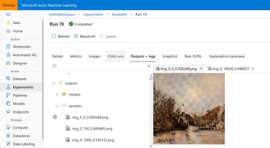
Getting Experiment Results

Once you are happy with results, it makes sense to get the results of the training in the form or model files and sample images. I have mentioned that during the training our training script stored models in outputs/models directory, and sample images - to outputs/samples. You can browse those directories in the Azure ML Portal and download the files that you like manually:

You can also do that programmatically, especially if you want to download all images produced during different epochs. run object that you have obtained during experiment submission gives you access to all files stored as part of that run, and you can download them like this:

run.download_files(prefix='outputs/samples')

This will create the directory outputs/samples inside the current directory, and download all files from remote directory with the same name.

I you have lost the reference to the specific run inside your notebook (it can happen, because most of the experiments are quite long-running), you can always create it by knowing the run id, which you can look up at the portal:

run = Run(experiment=exp,run_id='KeraGAN_1584082108_356cf603')

We can also get the models that were trained. For example, let's download the final generator model, and use it for generating a bunch of random images. We can get all filenames that are associated with the experiment, and filter out only those that represent generator models:

fnames = run.get_file_names()
fnames = filter(lambda x : x.startswith('outputs/models/gen_'),fnames)

They will all look like outputs/models/gen_0.h5, outputs/models/gen_100.h5 and so on. We need to find out the maximum epoch number:

no = max(map(lambda x: int(x[19:x.find('.')]), fnames))
fname = 'outputs/models/gen_{}.h5'.format(no)
fname_wout_path = fname[fname.rfind('/')+1:]
run.download_file(fname)

This will download the file with the highers epoch number to local directory, and also store the name of this file (w/out directory path) into fname_wout_path.

Generating new Images

Once we have obtained the model, we can just need load it in Keras, find out the input size, and give the correctly sized random vector as the input to produce new random painting generated by the network:

model = keras.models.load_model(fname_wout_path)
latent_dim=model.layers[0].input.shape[1].value
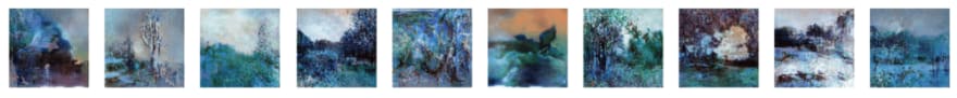
res = model.predict(np.random.normal(0,1,(10,latent_dim)))

Output of the generator network is in the range [-1,1], so we need to scale it linearly to the range [0,1] in order to be correctly displayed by matplotlib:

res = (res+1.0)/2
fig,ax = plt.subplots(1,10,figsize=(15,10))
for i in range(10):
    ax[i].imshow(res[i])

Here is the result we will get:

Have a look at some of the best pictures produced during this experiment:

Colourful Spring, 2020	Countryside, 2020
Through the Icy Glass, 2020	Summer Landscape, 2020

Subscribe to @art_of_artificial Instagram - I try to publish new pictures produced by GAN periodically.

Observing The Process of Learning

It is also interesting to look at the process of how GAN network gradually learns. I have explored this notion of learning in my exhibition Art of the Artificial. Here are a couple of videos that show this process:

Food for Thought

In this post, I have described how GAN works, and how to train it using Azure ML. This definitely opens up a lot of room for experimentation, but also a lot of room for thought. During this experiment we have created original artworks, generated by Artificial Intelligence. But can they be considered ART? I will discuss this in one of my next posts...

Acknowledgements

When producing keragan library, I was largely inspired by this article, and also by DCGAN implementation by Maxime Ellerbach, and partly by GANGogh project. A lot of different GAN architectures implemented in Keras are presented here.