Today I met Michael, who was confused about the car he had just serviced. The car broke down again and again. I don't know how often he had to service his vehicle because of the various conditions. After being traced, the service fees he has spent are equivalent to five times the purchase price of his car. Wow, fantastic, that car had to be replaced with a new car.
In addition to telling stories about how bad Michael's car was, he also asked me for advice on estimating how much it would cost for specific car criteria. So he can save diligently and have accurate goals. Without further ado, of course, I'm happy to help an old friend who accidentally met at a vehicle repair shop.
Maps to Help Michael
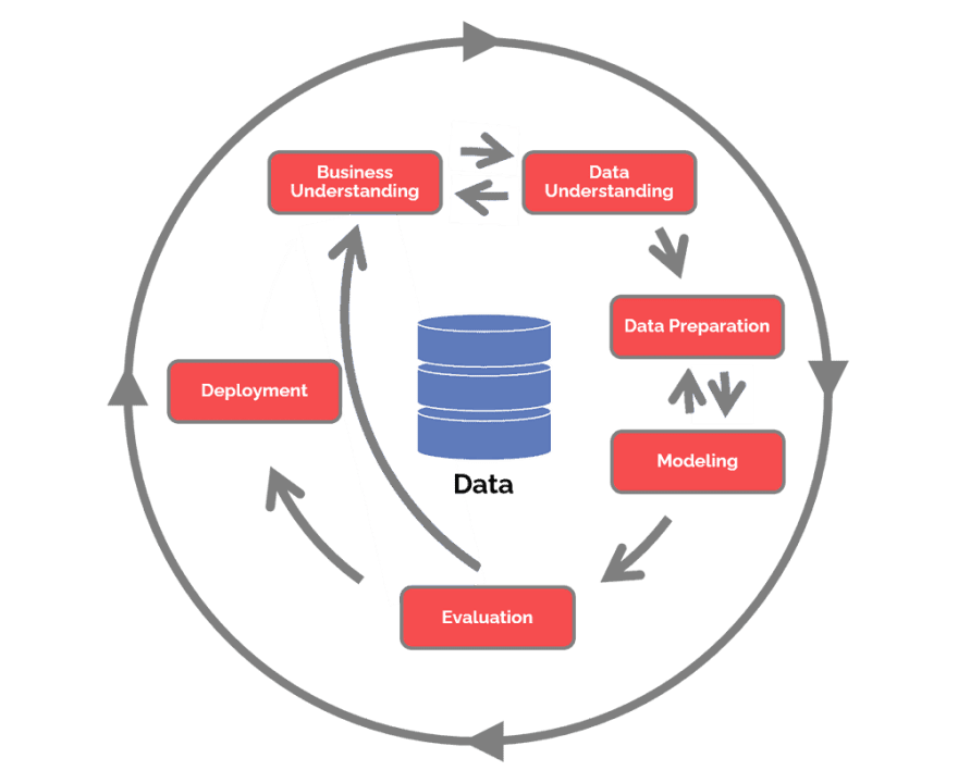
In helping Michael, I need a roadmap showing the end-to-end process of working on a data mining role regarding Estimation. Of course, I needed a framework called CRISP-DM, or the Cross-Industry Standard Process for Data Mining abbreviation. This framework seems to make it easier for us to help poor Michael. Here I present a series of processes used throughout the project to assist Michael.
Dataset Initiation
Before I get started, I need a bunch of price lists for cars where they come from. And luckily, I can get it directly at this link. In the dataset, I called 6019 types of car variations with 14 columns consisting of the car's characteristics and complete with the price of the vehicle. This dataset is big data and will probably represent the vehicle's overall price and help Michael set his savings goals later.
Business Understanding
This stage is the beginning to bring up the root of the problem. Luckily Michael has given an overview of the problem and needs help estimating the price of the car he wants in the future. I need a metric threshold to prove that the estimate is not too far off from the original data. I could use one of the metrics called Root Mean Squared Error (RMSE). At least I should get a relatively small RMSE value from an infinite RMSE range. That way, the average nominal variation of the estimated car price is not too far from the original price. OK, now to the Data Understanding stage.
Data Understanding
This stage shows a series of processes for exploring the dataset that we have obtained. Using cloud computing provided by Google (Google Colab), we will use the Python language to analyze the surface of our data.
1. Import equipment
We need some libraries and packages that are already available.
- We need Pandas for Data Frame analysis
- Numpy for array calculations and other operations
- Matplotlib and Seaborn for visualization of our analysis results

2. Upload dataset
Let's upload our dataset into an object called data and look at some examples of the data available there.

We can see that our dataset has 14 columns and 6019 rows of data. We need to look at each column's data distribution now.
3. Describing the dataset
We can describe the dataset we have by first removing the numeric and categorical type columns. This way, we can see the massive distribution of data.
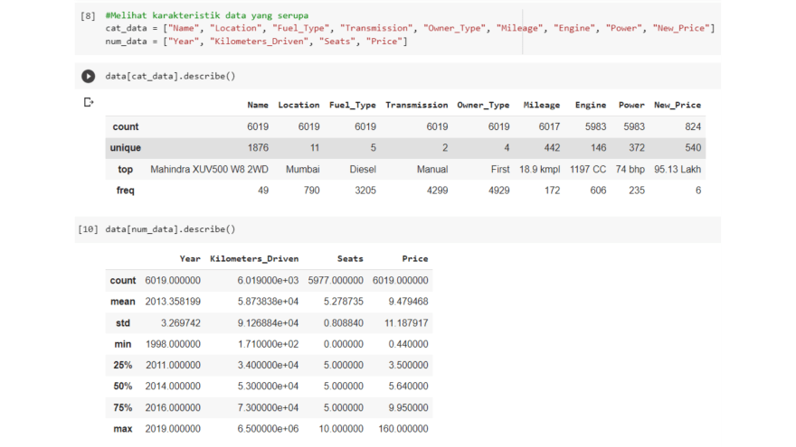
It seems that some of our numerical data are skewed in the data distribution. In addition, some columns should be numeric but become categorical data types in this case.
4. Something's amiss
We need to look at the distribution of our data with a histogram chart for numeric data. We have a bar chart for categorical data. It turns out that it varies significantly between the columns that we have!
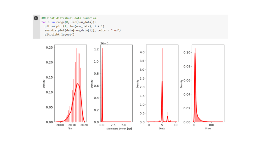
The Year column shows a negative trend while the Price column indicates a positive bias. The other two columns have too high a frequency of the same value and the same two values (bimodal). This oddness needs to be cleaned up by us later!

And yes, that's right, for categorical data, some of them have units that vary and make them of definite data type rather than numeric. But for some other columns, it's OK so far.
Data Preparation
Data preprocessing is the adjustment of the available columns to produce the best model. Based on the previous stages, the available dataset will be adjusted through several steps.
1. Handling missing values
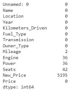
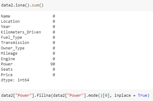
The data information we get shows an imbalance in the number of rows of data between several columns. This circumstance indicates missing observational data. Let's use data.isna().sum() to accumulate the amount of missing data.
Well, it turns out that there are several columns with missing values. As a consideration, let's delete the data row that contains the missing value. We might do this because the lost data is still below 10% of the total existing data.

However, for columns like Unnamed: 0 and also New_Price, it's best to delete the entire column.

2. Remove duplicate values
Duplicate data will undoubtedly bias a model because of its repetitive appearance. We can check whether exact data is available or not in this way.

Phew, luckily, our data has no duplicate values.
3. We must set outliers aside
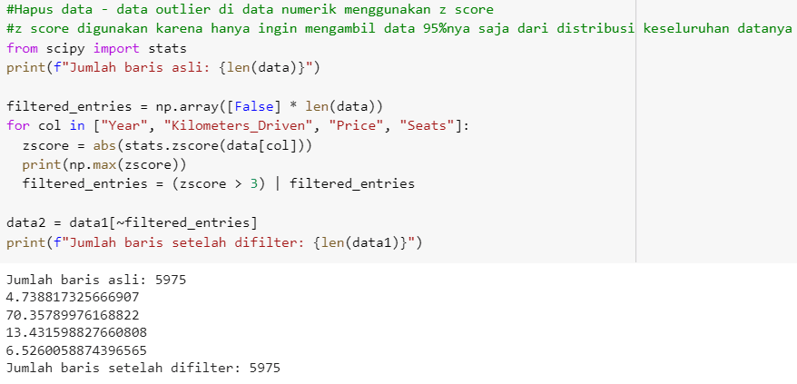
Do you remember the angular distribution of our numerical data? That data should clean immediately. This time, using the z-score value will be very helpful in taking the distribution of values as much as 95% of the quantity so that the numeric column we have will lose the super extreme weight.
Thankfully we only deleted 348 data. This consideration keeps our data representative of the population.
4. Heatmap shows your correlation!
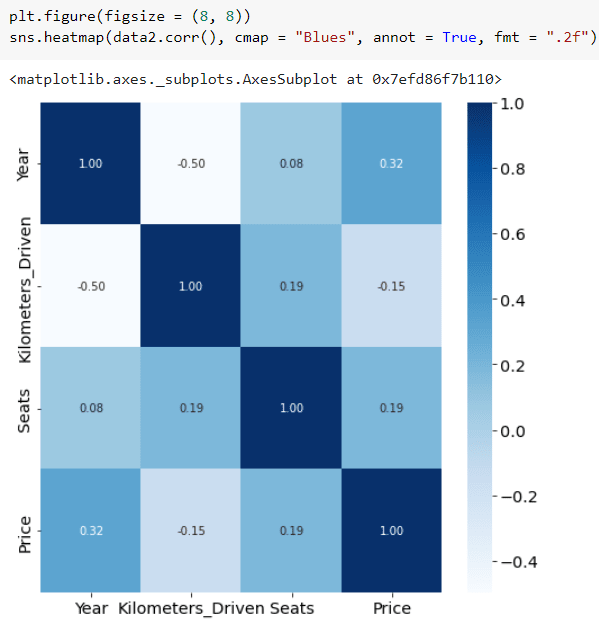
Heatmap will be very useful for seeing the Pearson correlation between several columns. The correlation heatmap available in seaborn renders the numeric columns as discrete values and crosses between the columns as the y-axis and the x-axis. This time we have to focus on our target column or the purpose of the estimation model we will make later.
From this, it can be seen that only the Year column, and even then, the correlation is only 0.23, which correlates with the Price target column. Our data needs further preprocessed by encoding categorical columns into numeric ones.
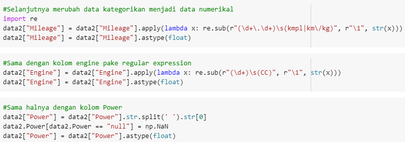
5. Regex in action
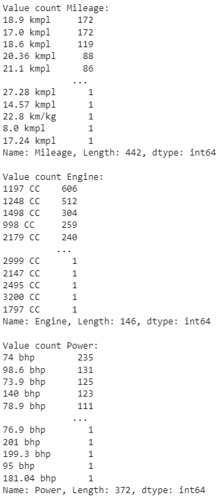
Regular expressions (regex) are crucial for customizing Mileage, Engine, and Power fields. The three columns are of numeric type, but because of the different units used, these columns are identified as categorical type columns. Let's look again at the three types of definite value types.
OK, that means we will delete each available unit and assume that one column has the same teams by taking only the cardinal values.
Note this: don't forget to change the column's data type to float. Because there are several values in the "null" Power column, it's time to delete the empty values that the previous null value has transformed.
6. Encode the rest!
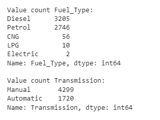
Look again at the available value variations in the Transmission and Fuel_Type columns!
The variation in the values in the two columns is not too much, and this is the right time to use One Hot Encoding. This technique will create new columns according to the variation of column values to be encoded. So the result is like this.
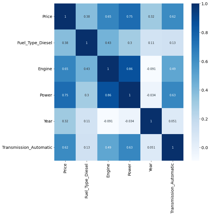
When all the columns have become one DataFrame, it's time to look at the heatmap correlation between attribute variables and classes from the preprocessed dataset.
From this, it can be concluded that several variables determine the price of a car, including:
- Diesel type fuel (Fuel_Type_Diesel)
- Strength of the engine (Engine)
- Available car power (Power)
- Year of the car (Year)
- Transmission type automatic (Transmission_Automatic)
Wrap it up into the model
It's time to make a suitable estimation model. For modeling, I will choose one machine learning algorithm, Random Forest, available in the SK-learn library. The stages in making the model will be divided into three processes.
1. Train and test with data
In teaching a data model, it is necessary first to divide it into two parts. So the Data Frame, which consists of six columns, is divided into training and test data. Also, make sure to separate the dependent variable as well as the independent variable, yes!
2. This car should be at this price.
Let's teach this model using training data in the following way.
When the model has learned from the available training data, it is time for it to be tested using data that has never been found before (aka data testing). Compare the overall estimation results with the previously split y_test data. Then the accuracy value of this model will be displayed as follows.
Well, that value is good enough as a benchmark for the estimated price of the new car that Michael will buy.
3. We need validation
Not necessarily that the model that has been created is ready to use. We must always validate whether the model has estimated the same value as the original data. We can do this by manually looking at the available test data. Then, we try to use the existing model by entering the value of the argument corresponding to the testing data.
Yes! the estimated price for the car is not too far away and is entirely accurate. Let's see whether our initial achievement has been met by evaluating some metrics.
Finally, Evaluation!
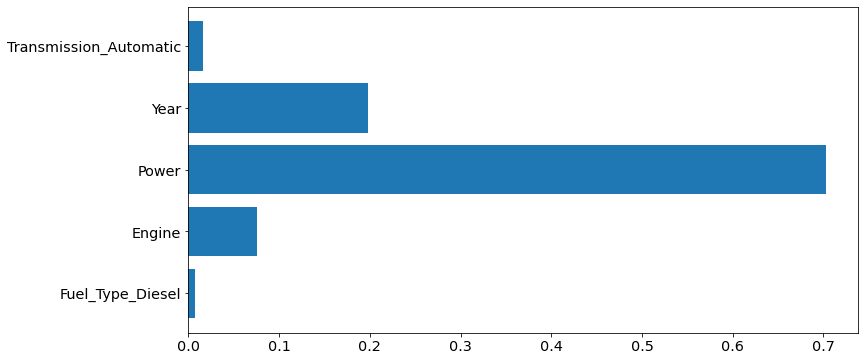
Evaluate, evaluate, evaluate! First, I'll show you what variables are the main determinants of how expensive a car can be.
It turns out that the Power variable is the culprit! I have to tell Michael that the higher the quantity of Power of a car, the higher the price of the vehicle will be. This insight will be a piece of helpful information for him. Of course, after I measured how successful this model was via the Root Mean Squared Error (RMSE) metric. RMSE is a metric that results from the root of the Mean Squared Error (MSE), which will show how much the average error value varies from the estimate given by this model. I will look at it this way.
Hooray! The RMSE results obtained by this model are too poor and adequately represent the accuracy value of the training data. It's time for me to meet Michael and talk about the insights I've found about him.







Top comments (16)
If you’re thinking “your car is costly!”, one of the first things I do when looking at pricier models is compare a bunch of listings to see what’s normal for that specific car. For example, if you’re interested in a used Mercedes GLA, browsing options from dealers like DRC Auto Sales Ltd gives you a real feel for what age, mileage and condition tend to cost on the market. It’s surprising how much prices can vary just from one example to the next, so seeing a range before you make a decision helps take some of the guesswork - and shock factor - out of it.
Greetings from Battstorm, your go-to source in Dubai, United Arab Emirates for expert vehicle battery replacement and repair services. Being a top garage which has best car battery replacement near me in the area, we are experts in offering quick, dependable, and superior auto battery replacements to keep your automobile in good operating order.
I can completely relate to Michael's frustration because I’ve been in a similar situation with an old blue car which I gave a funny name "dinky" that drained my wallet. It’s astonishing how quickly repair costs can pile up, especially when you’re dealing with recurring issues. In my case, I spent so much on engine repairs, brake replacements, and other fixes that I could have easily afforded a better, newer car if I had planned ahead. According to recent data, the average annual maintenance cost for a car can reach up to $1,000 or more, depending on the make and model, and unexpected breakdowns can cost thousands more. For example, replacing a blown engine alone can cost $5,000–$10,000. Looking back, I wish I had taken the time to estimate the total ownership costs of a new car instead of trying to keep an unreliable one alive. Michael is smart to start planning for a replacement now—it’s a lesson I learned the hard way!
It sounds like you had quite an adventure helping Michael estimate car prices using the CRISP-DM framework! I'm glad you could use data mining to provide accurate insights into car costs. It's fascinating how much detail you went into, from data preparation to model evaluation. Michael is lucky to have you help him set realistic savings goals. If you're interested in more tech-related content, feel free to check out my blog at germanic.ae/.
Interesting story! Poor Michael really did spend way too much on that old car. I think using CRISP-DM for estimating future costs makes a lot of sense starting with understanding the business need, preparing data on past service records, and then modeling to predict possible future expenses.
One thing I’ve noticed locally is that people sometimes overlook ongoing costs like paint protection, wraps, or window tinting, which can actually help save money by protecting the car’s interior and paint. For example, services like car tint san jose ca help reduce sun damage and keep the car cooler, lowering the need for frequent AC repairs and interior fixes.
Data-driven planning definitely helps set realistic savings goals and avoids surprises down the road. Thanks for sharing this roadmap it’s a useful reminder for anyone budgeting for car maintenance or upgrades!
I recently had my car serviced at Usman Autos and Services LTD in Grays, and I must say, it was a refreshing experience. As we all know, car maintenance can be expensive, but finding a trustworthy garage can make a significant difference.
Usman Autos offers a wide range of services, including MOTs, diagnostics, and general repairs. What sets them apart is their commitment to transparency and customer satisfaction. They don't upsell unnecessary services, which is a common concern among many drivers.
Their team is knowledgeable and approachable, providing clear explanations about the work needed and offering competitive pricing. It's evident that they value their customers and aim to build long-term relationships.
If you're looking for a reliable garage in the Grays area, I highly recommend giving Usman Autos a try. It's reassuring to know that there are still honest mechanics out there.
With a focus on "Gebrauchtwagen CH" and "Gebrauchtwagen," the website draws in visitors who are looking for premium used vehicles in Switzerland.
Some comments may only be visible to logged-in visitors. Sign in to view all comments.