pandas #3: Aggregation and Grouping

Let's continue with the series and learn more about how to analyse data with pandas. From the previous post we learned about reading files and basic DataFrame operations. Now we know how to store our data into a DataFrame object, so in this post we are going to do more with it.

Like the last post, this one will be more practical so I would appreciate if you code along with me. I try to do these posts independent from each other, here I'm considering that you'll create a new Jupyter Notebook, then I'm going to declare some variables again.

If you have any questions please feel free to use the comments section below.

Note [1]: I made a Jupyter Notebook available on my GitHub with the code used in this post.

Before we start

1. This is a pandas tutorial, then it's always required that we import pandas library in the beginning.
   

    import pandas as pd
   

2. Let's download the dataset we are going to work on.

   Note [2]: The file here is the same from my previous post, so if you have it already you can reuse it.
   

    !wget https://raw.githubusercontent.com/gabrielatrindade/blog-posts-pandas-series/master/restaurant_orders.csv
   

   

3. Now, let's turn it into a dataframe and store it in a variable.
   

    column_names = ['order_number', 'order_date',
                    'item_name', 'quantity', 'product_price']
   
    orders = pd.read_csv('restaurant_orders.csv', delimiter=',',
                         names=column_names)
   

If you would like to know details about this process, you can go through the previous post in Reading a File section.

Data Aggregation functions

First, we are going for more details about aggregations functions. But, what does it mean? and what is it for? Aggregate functions are used to apply functions in multiple rows resulting in one single value. By default, these functions are applied in each column (Series), so you can get a single value for each Series. Let me clarify this through our dataframe from the previous post. Do you remember the dataframe structure? Check it again.

orders.head()

And what if I wish to know how many records are in my data? Or how much I sold since I started to store my data? Or what about how many products did I sell? We can do this simply by summing all the numbers of a certain column (Series) or counting the number of lines in our dataframe, right?! But how to do that? Applying some aggregation functions we can get these numbers easily and get information like median, mean and so on.

sum()

Imagine that we would like to know how many products we sold, like I said before. We can do this by summing all the numbers from the quantity column, right?! Applying sum function directly on the column we can get the answer.

orders['quantity'].sum()

Note [3]: In the second post of this pandas series we saw how to access a value in column with pandas. If you go through the previous post (in Basic DataFrame operations >> Selecting specific rows and columns >> Columns) you can see that there are 3 ways to do that. You can compare the solution above with orders.quantity.sum() or orders[['quantity']].sum().

Note [4]: If you don't specify a column it will return the sum for each column of the dataframe.

In the same way, we can get numbers like how much I sold. But in this case we need to multiple the columns quantity and product_price before applying sum function.

(orders['quantity']*orders['product_price']).sum()

Note [5]: We use parenthesis to evaluate first the multiplication operation before doing the method call.

count()

Now, let's answer the question of how many records we have. To do this I need to count the number of lines I have in my dataframe. So, count function is appropriate for this case. As we did before, in this case we just apply the function over the dataframe.

orders.count()

However it will return the counting of records for each column.

As we can see each column has the same value. It happens because all columns (variables) were not empty. In case of None values, it would not be counted.

But if we want to get one unique value that represents the records quantity, we should choose a column which has no None values and apply the count function over it.

orders['order_number'].count()

min() and max()

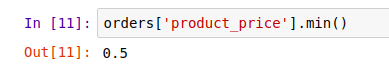
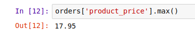
And what about the lowest product price I have recorded in my orders? Or the highest one? In these cases we are applying min and max functions, respectively, on the right Series (product_price).

orders['product_price'].min()

orders['product_price'].max()

mean() and median()

mean and median functions return us the column average and the column median, respectively. Below I briefly explain the difference between the two functions:

• mean() is the average of a set of numbers. To get this result just add all the numbers and then divide by the amount of elements you added. The mean is not a robust tool since it is largely influenced by outliers.
• median() is the middle value in an ascending ordered list of numbers. If the amount of elements in the list is even, i.e. has no middle number, so you add the two numbers in the middle and divide by 2 to get the median. The median is better suited for skewed distributions to derive at central tendency since it is much more robust and sensible.

Now, let's get the mean() and median() of quantity column.

orders['quantity'].mean()

orders['quantity'].median()

There are more aggregation functions, such as to calculate: standard deviation (.std()), variance (.var()), mean absolute deviation (.mad()), standard error of the mean of groups (.sem()), descriptive statistics (.describe()) and so on.

I would like to comment that through the describe function we can get a lot of information, like the ones already mentioned in this post, for example count, mean, median and std. But I'll show it in more details in a Data Wrangling post.

Grouping

Segmentation is part of a Data Scientist work. It means to separate the dataset in groups of elements which has something in common, or that makes sense to be in a group.

Let's take as an example our dataframe. In our dataframe we have records of products that were sold, right?! And it means that we have one or more records per order. So, what if we would like to know how many items were bought in each order? We should treat each order as a group and then apply sum aggregation function. Let's do it.

orders.groupby('order_number')[['quantity']].sum()

Note [6]: If I use just one bracket it will return a Series object, instead of DataFrame object. You can see more about this the previous post, in Basic DataFrame operations >> Selecting specific rows and columns >> Columns.

You can also put the Series you want to select in the end.

orders.groupby('order_number').sum()[['quantity']]

It won't make any difference in our result.

So... what about how many orders I have by day? It's another way that we can group our dataframe.

orders.groupby('order_date')[['order_number']].count()

Simple, isn't it?

Maybe you have noticed that a groupby call will usually be followed by an aggregation function. If we just groupby a dataframe without specifying the aggregation function, it will return the type pandas.core.groupby.DataFrameGroupBy object.

orders.groupby('order_number')

To practice more, let's get these values:

• The order with the highest amount of different products.

(orders.groupby('order_number')[['item_name']]
       .count()
       .sort_values('item_name', ascending=False)
       .head(1))

More details: sort_values function is sorting the result by item_name column, in descending order (ascending=False), then we get just the first result (head(1)).

• The 7 days that had the lowest quantity of products sold.

(orders.groupby('order_date')[['quantity']]
       .sum()
       .sort_values('quantity', ascending=True)
       .head(7))

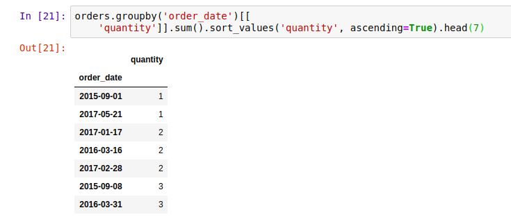
More details: Note that we changed to ascending order (ascending=True) because we want the days that have the lowest quantity of products sold.

• The 5 most expensive orders.

Before getting these 3 next answers, let's create a new dataframe with a subtotal column, which represents the product_price multiplied by quantity. To not damage our original dataframe, we can create one copy.

If you want to know more details, check the previous post (in Basic DataFrame operations >> Adding rows and columns >> Columns).

orders_copy = orders.copy()

orders_copy['subtotal'] = (orders_copy['product_price'] *
                           (orders_copy['quantity']))

Now, get the 5 most expensive orders.

(orders_copy.groupby('order_number')[['subtotal']]
            .sum()
            .sort_values('subtotal', ascending=False)
            .head(5))

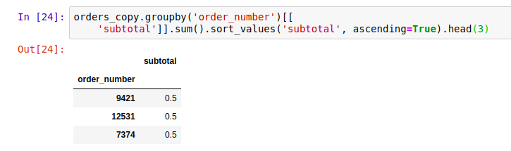
• The 3 cheapest orders.

(orders_copy.groupby('order_number')[['subtotal']]
            .sum()
            .sort_values('subtotal', ascending=True)
            .head(3))

• The 2 days that had the biggest income.

(orders_copy.groupby('order_date')[['subtotal']]
            .sum()
            .sort_values('subtotal', ascending=False)
            .head(2))

Wrapping up

This was the third post of pandas series. Here we learned about aggregation functions and grouping, and as you saw in some examples it's very useful and help us to discover new insights from our dataset.

Aggregation functions are used to apply specific functions in multiple rows resulting in one single value. And grouping is a way to gather elements (rows) that make sense when they are together. It's very common that we use groupby followed by an aggregation function.

I hope you enjoyed it and you found it clear. If you have any question, please let me know in the comments below.

In the next post we'll learn about merging.