1 - An Introduction to OpenJij

This project is still going. If you can help, please join in the OpenJij Slack Community. Then, you can participate in the project, and ask questions.

・OpenJij Slack

OpenJij is a heuristic optimization library of the Ising model and QUBO.
It has a Python interface, therefore it can be easily written in Python, although the core part of the optimization is implemented with C++.
Let's install OpenJij by pip. (Then, you need numpy.)

  []: !pip install openjij

  []: !pip show openjij # we assume openjij version is 0.0.5.

      Name: openjij
      Version: 0.0.5
      Summary: Framework for is model and QUBO
      Home-page: https://openjij.github.io/OpenJij/
      Author: Jij Inc.
      Author-email: [e-mail]
      License: Apache License 2.0
      Location: /usr/local/miniconda3/lib/python3.6/site-packages
      Requires: numpy, requests
      Required-by:

・The Ising model
The Ising model is a model treated in physics and is written as follows.

H({σ_i}) is called Hamiltonian, it is like an energy or a cost function.
σ_i is a binary variable it takes only two values ​​σ_i = -1 or 1.

Since σ_i corresponds to the physical quantity called spin in physics, it is sometimes called a spin variable or spin simply. Spin seems a micro magnet. The value of this variable corresponds to the physical state (the orientation of the magnet). σ_i = -1 means the magnet is up and 1 means magnet is down.

H depends on the combination of variables {σ_i}={σ_1, σ_2, ..., σ_N}.
Given J_ij and h_i represents the problem, and they are called interaction coefficients, longitudinal magnetic fields respectively.
OpenJij is a library which searches a combination of spin variables {σ_i} that minimizes H({σ_i}) when given J_ij and h_i.

Let me show you a concrete example.

・Let's try to solve a problem with OpenJij
We assume that the number of variables is N = 5, and the longitudinal magnetic field and interaction coefficients are

respectively.

In this case, since all interaction coefficients are negative, the energy is lower when each spin variable takes the same value.
Also, since all longitudinal magnetic fields are negative, the energy is lower when each spin takes 1.
Therefore, we can predict the answer of this problem is {σ_i} = {1, 1, 1, 1, 1}.

Now let's calculate using OpenJij.

  []:import openjij as oj

     # Create interaction coefficients and longitudinal magnetic fields that represent the problem.
     # OpenJij accepts problems in dictionary type.
     N = 5
     h = {i: -1 for i in range (N)}
     J = {(i, j): -1 for i in range (N) for j in range (i + 1, N)}

     print ('h_i:', h)
     print ('J_ij:', J)

    h_i: {0: -1, 1: -1, 2: 2: -1, 3: 1: 1, 4: -1}
    J_ij: {(0, 1): -1, (0, 2): -1, (0, 3): -1, (0, 4): -1, (1, 2): -1, (1 , 3): -1, (1, 4): -1, (2, 3): -1, (2, 4): -1, (3, 4): -1}

  []:# First, create an instance of Sampler to solve the problem.
    You can choose an algorithm to solve the problem by this selection.
    sampler = oj.SASampler()
    # Solve the problem(h, J) by using the method of sampler.
    response = sampler.sample_ising(h, J)

    # The result(state) of calculation is in result.states.
    print (response.states)

    # If you want to see the result with subscript, use response.samples.
    print (response.samples)

    [[1, 1, 1, 1, 1]]
    [{0: 1, 1: 2, 1: 3, 3: 1, 4: 1}]

・Explanation of OpenJij
Then, I will explain the code showed above.
OpenJij has two interfaces currently. One of them used above is the same interface as D-Wave Ocean.
Therefore, if you get used to using OpenJij, easy changing to Ocean.

Another interface will not be explained here, but it can be easily extended by using the structure of OpenJij(graph, method, and algorithm) directly. In the present situation, however, it would be sufficient to be able to use the interface which treated in the cell above.

・Sampler
Earlier, I created an instance of Sampler after creating the problem in the dictionary type.
sampler = oj.SASampler()
Here, this Sampler is the object of selecting what algorithm and hardware you use.
When you want to try the other algorithm, change this Sampler.

The algorithm treated in OpenJij is a heuristic and stochastic algorithm, it may return the different solutions each time the problem is solved, so it may not always obtain the optimal solution. Therefore, we solve the problem many times and search for a good solution. So we call Sampler which means that we sample the solutions.

SASampler treated in the above cell is a sampler that samples the solution by using an algorithm called Simulated annealing.
For example, we can choose other samples below.

• SQASampler: An algorithm for simulating quantum annealing called Simulated Quantum Annealing (SQA) with a classical computer.

• GPUSQASampler: It runs SQA on GPU. It can treat only a special structure called Chimera graph. Unstable.

・sample_ising(h, J)
When you want to solve the Ising model, you can use .sample_ising(h, J).
As I will explain later, when QUBO which equivalent to the Ising model optimization, use .sample_qubo(Q).

・Response
.sample_ising(h, J) returns the Response class.
This class contains results of solutions and energies that Sampler solved.

• .states:
  • type: list (list (int))
  • This list contains solutions to the number of iteration. > In physics, an array of spins called a state. Since .states stores the solutions to the number of iteration, we defined as .states from the meaning that multiple states are stored.

• .energies:
  • type: list (float)
  • This list contains the energy of each solution to the number of iteration.

• .indices:
  • type: list (object)
  • This list contains index of each spins corresponding to .states.

• .samples:
  • type: dict (key=index, value=variable value)
  • This dictionary contains states with index.

• .min_samples:
  • type: dict
  • This dictionary contains the keys 'min_states', 'num_occurences' and 'min_energy'. They are a list of states with minimum energy values, the number of times each state occurs, and minimum energy values respectively.

You can refer to the parameter listed above. It's hard to understand, so let's look at the code actually.

 []:# In fact, key h, J dictionaries can treat not only numbers.
    h = {'a': -1, 'b': -1}
    J = {('a', 'b'): -1, ('b', 'c'): 1}
    sampler = oj.SASampler(iteration = 10) # Try solving 10 times by SA at a time. With the argument called iteration.
    response = sampler.sample_ising(h, J)
    response.states

    [[1, 1, -1],
     [1, 1, -1],
     [1, 1, -1],
     [1, 1, -1],
     [1, 1, -1],
     [1, 1, -1],
     [1, 1, -1],
     [1, 1, -1],
     [1, 1, -1],
     [1, 1, -1]]

You can see that the response.states contains 10 solutions when you open it.
Since this problem is easy, returned the same answer is [1, -1, 1] every iterations.
Next, let's look at the energies.

  []:response.energies

     [-4.0, -4.0, -4.0, -4.0, -4.0, -4.0, -4.0, -4.0, -4.0, -4.0, -4.0]

Of course, the energies also take the same value every iterations.
The solutions in response.states are list type, so you confuse the corresponding to the strings a, b, c when you set the problem.
That is in response.indices.

  []:response.indices

     ['a', 'b', 'c']

If you want to link the index and the state, use dict(zip(response.indices, response.states[0])) or call .samples.

 []:response.samples

    [{'a': 1, 'b': 1, 'c': -1},
     {'a': 1, 'b': 1, 'c': -1},
     {'a': 1, 'b': 1, 'c': -1},
     {'a': 1, 'b': 1, 'c': -1},
     {'a': 1, 'b': 1, 'c': -1},
     {'a': 1, 'b': 1, 'c': -1},
     {'a': 1, 'b': 1, 'c': -1},
     {'a': 1, 'b': 1, 'c': -1},
     {'a': 1, 'b': 1, 'c': -1},
     {'a': 1, 'b': 1, 'c': -1}]

When you need know only the solution which has the lowest energy, .min_samples is useful.
Note that min_samples['min_states'] have multiple solutions if the solutions are degenerate.

Degeneracy: Different solutions (states) have the same energy value (cost value)

 []:response.min_samples

    {'min_states': array([[1, 1, -1]]),
     'num_occurrences': array([10]),
     'min_energy': -4.0}

・Let's try to solve the QUBO
When you want to solve social problems,
it is often easier to formulate as QUBO(Quadratic Unconstraited Binary Optimization) than the Ising model.
Basically, it returns the same solution when using the Ising model.

QUBO is written as follows.

Binary variables take 0 or 1, that is difference between QUBO and Ising model.
There are other ways to define ∑ and Q_ij (for example, make Q_ij a symmetric matrix),
but in this time we have formulated it as above.

The Ising model and QUBO are equivalent for the reason why they can be converted to each other. You can convert these equations: q_i = (σ_i + 1)/2.

In the case of QUBO, you search a combination of {q_i} that minimizes H({q_i}) under the Q_ij which is given by a problem.
It is almost the same as the Ising model.

Also, since q_i^2 = q_i (because q_i takes only 0 or 1), you can write as follows.

Namely, the diagonal components of Q_ij is corresponds to the coefficients of the first-order term of q_i.

Let's solve with OpenJij.

    []:# Create Q_ij in dictionary type.
       Q = {(0, 0): -1, (0, 1): -1, (1, 2): 1, (2, 2): 1}
       sampler = oj.SASampler(iteration = 3)
       # Use .sample_qubo when you solve the QUBO.
       response = sampler.sample_qubo(Q)
       response.states

       [[1, 1, 0], [1, 1, 0], [1, 1, 0]]

In QUBO, the solutions are made by 0 or 1 because the variables take 0 or 1.
OpenJij can solve the optimization problem of the Ising model and QUBO.

・Let's solve a little difficult problem
You want to solve a problem of QUBO which has Q_ij given by 50 random variables.

    []:N = 50
       # Create Q_ij randomly
       import random
       Q = {(i, j): random. Uniform (-1, 1) for i in range (N) for j in range (i + 1, N)}

       # Solve by OpenJij
       sampler = oj.SASampler(iteration = 100)
       response = sampler.sample_qubo(Q)

    []:# Look at some energies.
       response.energies[: 5]

       [-46.435277356769575,
        -46.435277356769575,
        -45.99099675164143,
        -46.38082975608086,
        -45.96001255429061]

You will realize that the energies takes a different values than before.
If you make Q_ij randomly, the problem becomes difficult generally.
Therefore, SASampler does not necessarily give the same solution every time.
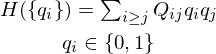
Now let's look at the histogram of energies.

    []:import matplotlib.pyplot as plt
       plt.hist(response.energies, bins = 15)
       plt.xlabel('Energy', fontsize = 15)
       plt.ylabel('Frequency', fontsize = 15)
       plt.show()

The lower the energy, the better, but you can find that the high energy solutions appear sometimes.
However, almost half of them seem to have the lowest energy.

Openjij solved the problem 100 times.
Since the optimal solution is the lowest energy,
the lowest energy solution among the solved (sampled) solutions should be close to the optimal solution.
Therefore, we search for the solution from .states.

Caution!: SA can not always give an optimal solution.
Therefore, there is no guarantee that the solution with the lowest energy in this time is an optimal solution.
It is an approximate solution.

    []:import numpy as np
       min_samples = response.min_samples
       min_samples

       {'min_states': array ([[0, 1, 0, 1, 1, 1, 1, 1, 1, 1, 1, 0, 0, 0, 1, 1, 0, 1, 1, 1 , 1,
                0, 1, 1, 0, 0, 1, 0, 1, 0, 1, 1, 0, 1, 1, 0, 1, 0, 1, 0, 0, 0, 1,
                1, 0, 1, 0, 0, 1]],
        'num_occurrences': array([17]),
        'min_energy': -46.44424507437836}

Now you get the lowest energy solution.
The solution which is contained in this min_states is the approximate solution in this time.
Contained solutions have the same energy,
but the arrangement of spins may differ in some cases (In the case of "degenerated state").

So, after choosing the lowest energy state as above, choose the spin orientation from min_state as you like.
Then, we solved the problem approximately.

Next section, “2-Evaluation”, we will explain the index("time to solution" and "the residual energy" etc.) for evaluate the solution.

If you have any questions, please join in the Slack Community.
・OpenJij Slack