
Note: Spanish translation of this article: leer en español | Last updated: 09/01/25
In this article, you will learn about geospatial data for developers.
If you have ever tried to:
- Display an open dataset with "strange" coordinates.
- Store complex geographical shapes in a regular database.
- Display thousands of locations on an interactive map.
- Figure out which ones fall inside a specific area.
- Calculate distances between them.
You’ve already bumped into the unique challenges of working with geospatial data.
You maybe even ended up writing too much code to account for these challenges, or found your app slowing down due to the complexity in dealing with these complex datasets.
From my 10+ years of experience helping developers get started with geographic information systems (GIS), I’ve come to realize that most computer science degrees and coding bootcamps don’t cover this topic at all.
As a result, many developers try to handle location data using the same tools and mindset they would use for any other kind of data, until they find limitations, the logic becomes painfully complex, or things stop scaling.
In this article, I’ll explain why working with geospatial data involves much more than just “data with coordinates,” and why specialized technologies (such as spatial databases, geospatial servers, APIs, and mapping SDKs) are essential to your work.
Table of contents:
- Why geospatial data needs a different mindset
- How spatial data is structured
- Querying and analyzing
- Geospatial data integrity
- Performance strategies
- Visualization and User Experience
- Interoperability
- Geospatial APIs
- Takeaways
Why geospatial data needs a different mindset
Think of it like this: most of the time, you’re still working with tables (rows and columns), but each row includes one or more coordinates that define where in the world that data lives. Sometimes it’s a single point, other times, it’s a line or polygon that outlines a route or a region.
And here’s the catch: this location data shouldn’t just be stored as a regular field like a string or a float. It requires specialized spatial field types, because you’ll want to do operations that standard data types or SQL queries cannot handle efficiently.
How spatial data is structured
To work effectively with geospatial data, you need to understand the various shapes it can take, because how you model location affects how you store, query, and use it.
In many ways, it’s like choosing the right data structure for a problem: different shapes represent different kinds of real-world things and require different logic under the hood.
Here are two fundamental distinctions to know.
Discrete vs continuous data
Not all location data works the same way. Some datasets describe discrete objects (also known as geometries or vector data), things with clear boundaries, such as store locations, building footprints, roads, or property lines. You can think of these as the “objects” in the spatial world: they exist in one place and have a shape that has a well-defined boundary that can be represented with a JSON.
Other datasets are continuous, like elevation, temperature, or noise levels, values that vary across space without distinct edges. These are more like gradients, and you can’t model them with a simple shape. Instead, they’re typically stored as raster data, grids of values where each cell represents a measurement at a specific location, and require different tools for analysis and visualization.

Before we move on, let me clarify the difference between discrete objects, geometries, and vector data. While related, they are not the same:
Discrete objects: what you’re modeling conceptually (e.g., roads, parcels, trees, rivers, buildings).
Geometries: the shape of those objects, their technical/mathematical representation (point, line, polygon), defined by coordinates that describe their position and boundaries in space.
Vector data: the data structure used to store and manage them in GIS (e.g., GeoJSON, shapefiles, feature services, or vector tiles).
When discussing the structure of spatial data, it’s important to separate two closely related but distinct ideas: the data model used to represent it (vector vs. raster) and the type of phenomenon (discrete vs. continuous).
Discrete phenomena have clear boundaries, such as roads, parcels, or categories like land cover classes.
Continuous phenomena vary gradually across space, like elevation or temperature.
Either phenomenon type can be stored as a vector or a raster. For instance, land cover is conceptually discrete but often represented as a raster grid of classes, while elevation is continuous but can also be expressed as vector contour lines.
Keeping these two dimensions separate helps avoid the common misconception that “discrete = vector” and “continuous = raster.
⚠️ Disclaimer: To keep things simple, the rest of this article will primarily cover how vector datasets representing discrete objects should be managed. While raster datasets are equally important in geospatial work, they present different challenges that are beyond the scope of this introduction; therefore, we will not cover them here.
Discrete geometry types
The most common geometries to represent discrete datasets are:
- Points: A single pair of coordinates (like a coffee shop or delivery drop-off).
- Lines (also known as polylines): A sequence of points forming a path (like a walking route or a river).
- Polygons: A closed shape that defines an area (like a park or postal code).
However, there are also more complex geometry types, such as multipoints, curved lines, and polygons with curved edges or holes. In 3D contexts, you may also work with 3D objects, such as meshes or voxels, which represent surfaces, volumes, or real-world structures in three dimensions.
These aren’t just visual elements; they define how you’ll query, intersect, or join spatial data. And they also affect performance, precision, and indexing strategies, which is why they’re treated as native field types in spatial databases.
Querying and analyzing
Once your data includes location, you can go far beyond standard filtering or joins. Spatial databases extend SQL with operations that let you analyze how things relate in space and provide mechanisms to enforce spatial integrity.
Let’s explore some of these capabilities.
Spatial relationships (predicates)
These are Boolean operations that evaluate the relationship between two geometries in space. They don’t produce new geometries; they just return true/false or are used in filters/joins.
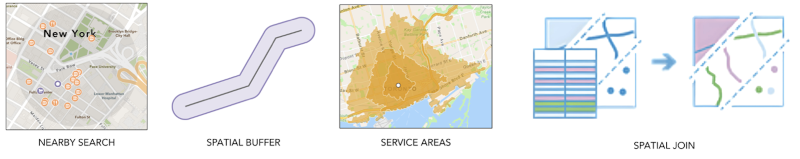
For example, in a traditional database, you might join tables by ID or name. However, in a spatial database, you can join rows based on their location (spatial joins), allowing you to join data by spatial proximity rather than keys.
Example of the intersect operation between different geometry types:

Find more at: Types of geometry operations.
Spatial operations (transformations)
These generate new geometries as output, often used in analysis or visualization workflows:
Examples include:
- Buffering: for proximity searches (creating areas around coordinates or shapes).
- Unions: combine several geometries.
- Intersection: is a property within a restricted zone?
- Service areas: find reachable zones in X minutes.
Another powerful spatial operation is tessellation, which means dividing space into regular, non-overlapping shapes that cover an area completely (commonly squares, hexagons, or triangles).
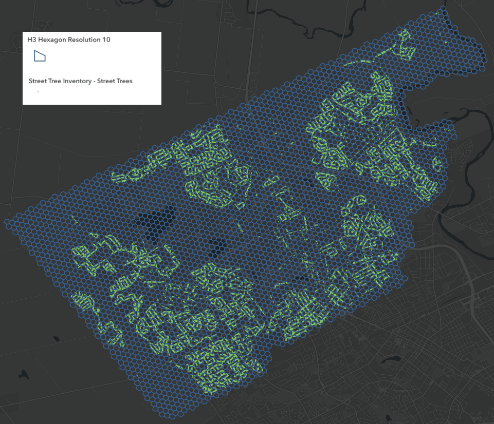
Tessellations are widely used in spatial analysis to standardize how data is aggregated and compared across regions. Beyond analysis, tessellation also plays a key role in user experience and performance.
Learn more about spatial analysis and how to use tesselation.
Spatial measurements
Not all spatial operations return shapes or yes/no answers; sometimes, what you need is a number, whether you’re calculating the distance between two points, the area of a polygon, or the length of a path.
These operations return quantitative values and are essential for sorting results, displaying meaningful stats, or supporting ranking and filtering logic in your apps.
Some use cases include:
- Distance calculations: Compute the shortest distance between two geometries (e.g., how far a user is from the nearest store or point of interest).
- Area and perimeter: Measure the surface area of a polygon (e.g., parcel size).
- Line length: Calculate the total distance along a route or path.
- Geodesic vs planar measurements: Many tools support both planar (flat-earth) and geodesic (earth-curved) calculations, which can significantly affect accuracy over large distances or near the poles.
Geospatial data integrity
Before performing any meaningful spatial analysis, it’s essential to ensure that the data is accurate, as spatial errors are easy to introduce. Common issues include overlapping polygons, gaps between parcels, or disconnected road segments, all of which can compromise the validity of your analysis.
Just as you define NOT NULL, foreign keys, or uniqueness constraints in a traditional schema, geospatial systems enable you to define topology rules that enforce spatial correctness.
For example:
- No overlaps allowed: useful for land parcel boundaries.
- Must be within another shape: e.g., buildings must be inside property zones.
- Lines must connect at endpoints for routing networks.
These rules help maintain data quality and prevent logic errors in downstream apps, maps, or analyses.

Performance strategies
Now that we’ve covered how spatial data is stored, queried, and analyzed, it’s time to focus on the next challenge: efficiently working with large and complex geospatial datasets.
As the volume and complexity of spatial data grow, so do the performance demands, and solving them requires more than just faster hardware. We need to apply specialized techniques and strategies that account for the unique nature of spatial operations.
Here are some of the key techniques, like spatial indexing, geometry simplification, and tiling, that make responsive, scalable geospatial apps possible.
Spatial indexing
Some geospatial datasets can easily contain thousands or millions of shapes, ranging from small collections of local objects to datasets that cover vast areas, such as countries, intergovernmental regions, transoceanic zones, or even the entire world. These shapes may include thousands of vertices, making them complex to process.
To run fast spatial queries (e.g., intersects, within), spatial databases use specialized spatial indexes like R-trees. These indexes organize geometries by their bounding boxes, enabling the system to quickly filter out irrelevant areas, much like how B-tree indexes help accelerate range queries in traditional databases.
Without spatial indexing, even simple queries would require scanning every geometry, which quickly becomes unmanageable at scale.
How do spatial indexes work?
Spatial indexes work by simplifying complex geometries into bounding boxes (rectangular envelopes that fully contain each shape). Take a look at the following image, which illustrates how spatial indexes work:

In the illustration, each feature (A, B, C, and D) is enclosed by a bounding box, which is what the spatial index stores, not the full geometry.
If we want to know which shapes intersect with feature A (the area around the marker), the spatial index performs a fast initial filtering step. It identifies all features whose bounding boxes intersect with A’s bounding box. In this case, B and D are potential matches.
This step avoids checking geometries that are clearly irrelevant (like C), improving performance significantly.
Then, in a second phase, the database performs a precise geometric check on the candidate features (B and D) to verify actual intersections.
This two-step process: bounding box filtering followed by exact geometry comparison, is what makes spatial queries efficient, especially when dealing with large and complex datasets.
Simplification and tiling
This is about delivering data at the right level of detail. When you build a map application, users will pan and zoom. The same dataset that looks fine when zoomed in can become overwhelming and difficult to render efficiently when zoomed out.
To keep things fast, you need to adapt the data dynamically:
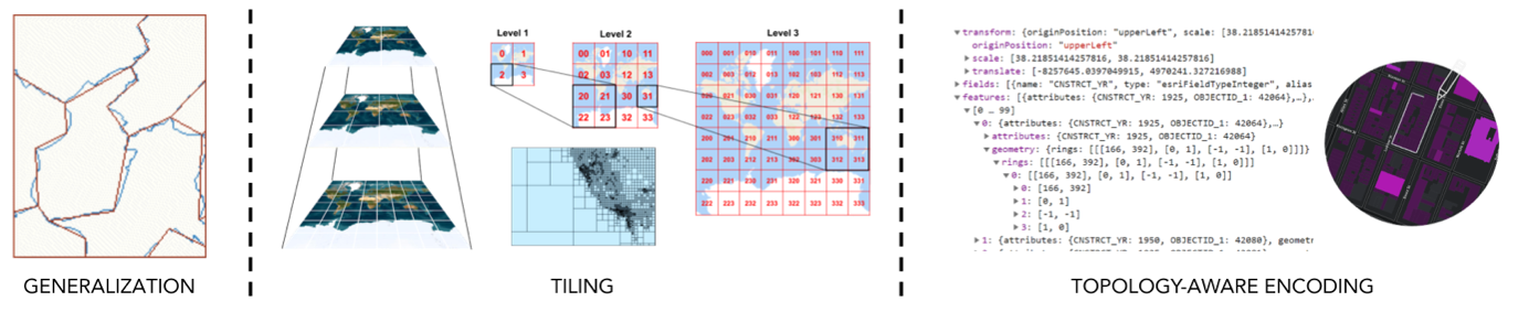
- Simplify geometries: Just like responsive design adapts to screen sizes, maps need to adapt detail to scale. This is done by reducing the number of vertices in a shape as the user zooms out, a process known as generalization.
- Tile the data: Geospatial systems often split data into tiles, small chunks representing a specific area and zoom level. This is like lazy-loading components in a frontend app: only load what you need, when you need it. Tiling lets you render massive datasets progressively, keeps memory usage low, saves bandwidth, and speeds up load times.
- Compress with topology-aware encoding: reduce file size by encoding shared boundaries only once and storing coordinates as deltas from previous points. This minimizes redundancy and ensures topological consistency between adjacent shapes, making data smaller and cleaner for delivery.
Without simplification and tiling, rendering large geospatial datasets would quickly become a bottleneck. You’d be forced to load entire layers into memory, process overly detailed geometries at every scale, and deal with slow rendering, high bandwidth usage, and unresponsive user interfaces.
Visualization and User Experience
Maps are often the primary interface for interacting with geospatial data, and how that data is visualized can make or break the user experience. Clear, performant map design depends on techniques like scale-based visibility, proper symbolization, and more.
Client-side mapping technologies
To work effectively with spatial data and build fast, interactive, and insightful geospatial applications, you need specialized mapping tools.
These tools need to be optimized to:
- Render rich, data-driven visualizations: Support both continuous and discrete data, with the ability to symbolize 2D and 3D geometries using dynamic styles. Visualize spatial data through heatmaps, clusters, geolocated pie charts, and more. Provide curated libraries of cartographic symbols for common use cases (points of interest, transportation, boundaries, etc.) so you don’t need to design everything from scratch.
- Manage spatial references and projections: Support rendering maps in various coordinate systems, and reproject data on-the-fly to ensure spatial accuracy and consistency across layers (we’ll cover spatial references in more detail below).
- Perform client-side spatial analysis: Enable real-time operations such as distance calculations, buffering, spatial joins, and geometry processing, directly in the client.
- Ensure performance at scale: Handle large datasets efficiently using the tile-based rendering, topology-aware geometry compression, and hardware acceleration through WebGL, WebGPU, Web Workers, and other performance enhancements.
- Provide prebuilt UI widgets and interaction tools: Offer customizable, ready-to-use components like zoom controls, search bars, legends, measurement tools, sketch editors, popups, and more, accelerating UI development.
- Support interoperability and extensibility: Work seamlessly with widely adopted geospatial standards such as GeoJSON, WMS, WMTS, 3D Tiles, or COG. Some of these are defined by the OGC, the geospatial equivalent of the W3C. These tools should also let developers add custom layers or renderers and extend functionality (e.g., through a plugin-friendly architecture).
Without client-side mapping technologies, you’d end up reinventing the wheel, manually building performance optimizations, drawing logic, interactive behaviors, and UI components that these tools already handle for you.
Development and cartographic design tools
Building great maps isn’t just about code. Great user experiences depend not only on data and logic, but also on how that data is styled, labeled, and presented across different scales and contexts.
A good development experience requires tools that make it easier to design, develop, test, and refine cartographic styles without starting from scratch.
These tools accelerate development and improve design quality by enabling:
- Data exploration: Inspect spatial data visually to understand distributions, outliers, or gaps, helping you make better styling and filtering decisions early in the workflow.
- Visual style editors and map builders: Quickly experiment with map designs (symbols, layers visibility, labels, popups, and more) using interactive GUIs with live preview. This saves time during design iteration.
- Custom symbol builders: Create symbols visually (e.g., advanced markers) using visual tools.
- Style import/export: Save and reuse visual styles across projects or environments. Load styles dynamically from the client SDK to reduce code and ensure consistent map design across teams and apps.
An example of this type of data exploration, map authoring, and even analysis tool would be the ArcGIS Map Viewer.:

And an example of a cartographic design tool is the Vector Tile Style Editor:

Without development and cartographic design tools, every visual change would require manual code edits, refresh cycles, and trial-and-error guessing. You’d waste valuable time tweaking styles without visual feedback, struggle to maintain consistency across projects, and overload developers with work that designers could handle more efficiently through visual tools.
Interoperability
As with any software system, interoperability within a geospatial system also matters. This section highlights the importance of spatial references, file formats, and API specifications when integrating and working across systems.
Spatial references
There’s no single universal way to represent location. The most widely known system used by GPS and expressed in latitude and longitude is known as WGS84. But many datasets, especially from open data portals or government agencies, use other spatial reference systems like UTM or Web Mercator, which express positions differently (e.g., in meters instead of degrees).
Although spatial references ensure interoperability, they also play a crucial role in ensuring accuracy. Just like mixing text encodings (UTF-8 vs ISO-8859-1) can cause characters to display incorrectly, mixing spatial data with different coordinate systems without reprojection can cause features to appear in the wrong place, or not show up at all.
The following image illustrates how the same coordinates expressed in two different systems represent different locations on Earth.
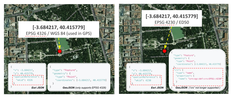
If you want to know more about this, you can check Spatial references in our developer docs.
Geospatial data formats
All geospatial file formats define the spatial reference of the data (either explicitly or implicitly) along with the geometry itself. Well-known formats like GeoJSON, Esri JSON, TopoJSON, GeoPackage, and Shapefile are designed to carry not just raw coordinates, but also essential metadata.
Unlike plain CSVs that may contain coordinates but lack spatial context, these formats embed critical information such as spatial references, attribute schemas, and projection details, ensuring the data is accurately interpreted, styled, and integrated across different systems.
Geospatial APIs
To make it easier to discover and interact with such data via APIs, there are well-established open specifications explicitly designed for geospatial content. These include OGC standards like WMS, WFS, and OGC API, as well as our ArcGIS REST APIs and STAC.
These APIs typically expose:
- Service metadata (e.g., name, description, provider, license)
- Available layers or feature collections
- Supported spatial reference systems
- Supported output formats
- And other technical capabilities that make the data easier to explore, visualize, or analyze across different systems.
For developers, understanding geospatial APIs is key not only to saving valuable development time (by leveraging existing tools and workflows instead of reinventing them) but also to building interoperable solutions that work across different platforms. By following well-known specifications, these APIs provide consistent access to spatial data, reducing the need for custom parsing, manual conversions, or coordinate fixes.
Takeaways
As we have seen, geospatial data isn’t just “data with coordinates”. Working with location data presents unique challenges that require new tools and ways of thinking. So, if you’ve ever struggled with location data, now you know why.
The good news? There’s a whole ecosystem of tools built to help you. To address them, you can embrace the tools explicitly built to work with geospatial data, such as spatial databases, geospatial servers, client-side SDKs, and specialized cartographic design tools, and you’ll save time and headaches.
What’s next? If you’d like to dive deeper, I recommend exploring our developer guides and the Interactive Learner GIS. If you’re interested in hosted cloud services, I’ve also started a blog series that breaks down ArcGIS hosted services in detail (feature services, vector tile services, and map tile services).
And if you find something confusing or believe you’ve spotted an error or inconsistency in this article, we’d love to hear from you. Please reach out to us at developers@esri.com so we can ensure the content remains clear, accurate, and insightful.
If you found this article helpful and believe others in your professional network may benefit from it, we would greatly appreciate it if you could share or engage with the post on LinkedIn, Bluesky, or X.

Top comments (2)
🥳🎉
😍