Class imbalance and classification metrics with aircraft wildlife strikes ✈️

This is the latest in my series of screencasts demonstrating how to use the tidymodels packages, from just starting out to tuning more complex models with many hyperparameters. I recently participated in SLICED, a competitive data science prediction challenge. I did not necessarily cover myself in glory but in today’s screencast, I walk through the data set on aircraft wildlife strikes we used and how different choices around handling class imbalance affect different classification metrics.

Here is the code I used in the video, for those who prefer reading instead of or in addition to video.

Explore data

Our modeling goal is to predict whether an aircraft strike with wildlife resulted in damage to the aircraft. There are two data sets provided, training (which has the label damaged) and testing (which does not).

library(tidyverse)

train_raw <- read_csv("train.csv", guess_max = 1e5) %>%
  mutate(damaged = case_when(
    damaged > 0 ~ "damage",
    TRUE ~ "no damage"
  ))
test_raw <- read_csv("test.csv", guess_max = 1e5)

There is lots available in the data!

skimr::skim(train_raw)

Name	train_raw
Number of rows	21000
Number of columns	34
_______________________
Column type frequency:
character	20
numeric	14
________________________
Group variables	None

Table 1: Data summary

Variable type: character

skim_variable	n_missing	complete_rate	min	max	empty	n_unique	whitespace
operator_id	0	1.00	3	5	0	276	0
operator	0	1.00	3	33	0	275	0
aircraft	0	1.00	3	20	0	424	0
aircraft_type	4992	0.76	1	1	0	2	0
aircraft_make	5231	0.75	2	3	0	62	0
engine_model	6334	0.70	1	2	0	39	0
engine_type	5703	0.73	1	3	0	8	0
engine3_position	19671	0.06	1	11	0	4	0
airport_id	0	1.00	3	5	0	1039	0
airport	34	1.00	4	53	0	1038	0
state	2664	0.87	2	2	0	60	0
faa_region	2266	0.89	3	3	0	14	0
flight_phase	6728	0.68	4	12	0	12	0
visibility	7699	0.63	3	7	0	5	0
precipitation	10327	0.51	3	15	0	8	0
species_id	0	1.00	1	6	0	447	0
species_name	7	1.00	4	50	0	445	0
species_quantity	532	0.97	1	8	0	4	0
flight_impact	8944	0.57	4	21	0	6	0
damaged	0	1.00	6	9	0	2	0

Variable type: numeric

skim_variable	n_missing	complete_rate	mean	sd	p0	p25	p50	p75	p100	hist
id	0	1.00	14980.94	8663.24	1	7458.75	14978.5	22472.25	30000	▇▇▇▇▇
incident_year	0	1.00	2006.06	6.72	1990	2001.00	2007.0	2012.00	2015	▂▃▅▆▇
incident_month	0	1.00	7.19	2.79	1	5.00	8.0	9.00	12	▃▅▆▇▆
incident_day	0	1.00	15.63	8.82	1	8.00	15.0	23.00	31	▇▇▇▇▆
aircraft_model	6259	0.70	24.65	21.70	0	10.00	22.0	37.00	98	▇▆▂▁▁
aircraft_mass	5694	0.73	3.50	0.89	1	3.00	4.0	4.00	5	▁▁▂▇▁
engine_make	6155	0.71	21.22	11.04	1	10.00	22.0	34.00	47	▇▂▆▇▁
engines	5696	0.73	2.05	0.46	1	2.00	2.0	2.00	4	▁▇▁▁▁
engine1_position	5838	0.72	2.99	2.09	1	1.00	1.0	5.00	7	▇▁▂▅▁
engine2_position	6776	0.68	2.91	2.01	1	1.00	1.0	5.00	7	▇▁▂▅▁
engine4_position	20650	0.02	2.02	1.43	1	1.00	1.0	4.00	5	▇▁▁▃▁
height	8469	0.60	819.24	1772.53	0	0.00	50.0	800.00	24000	▇▁▁▁▁
speed	12358	0.41	141.39	52.25	0	120.00	137.0	160.00	2500	▇▁▁▁▁
distance	8913	0.58	0.66	3.33	0	0.00	0.0	0.00	100	▇▁▁▁▁

The data is imbalanced, with not many incidents resulting in damage.

train_raw %>%
  count(damaged)


## # A tibble: 2 x 2
## damaged n
## <chr> <int>
## 1 damage 1799
## 2 no damage 19201

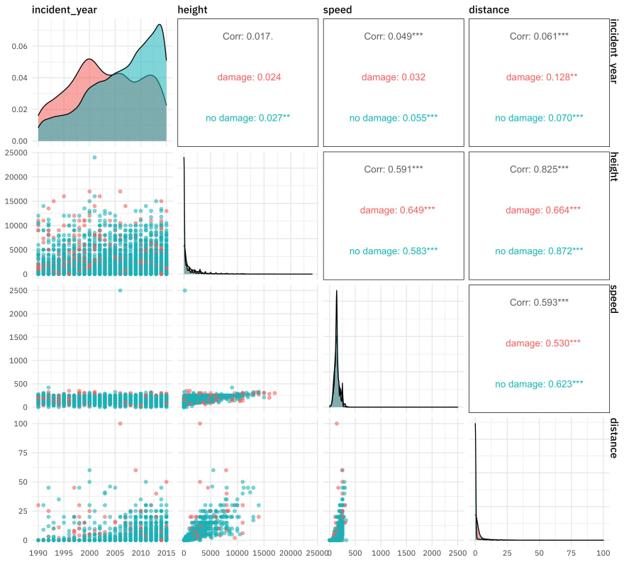
For numeric predictors, I often like to make a pairs plot for EDA.

library(GGally)

train_raw %>%
  select(damaged, incident_year, height, speed, distance) %>%
  ggpairs(columns = 2:5, aes(color = damaged, alpha = 0.5))

For categorical predictors, plots like these can be useful. Notice especially that NA values look like they may be informative so we likely don’t want to throw them out.

train_raw %>%
  select(
    damaged, precipitation, visibility, engine_type,
    flight_impact, flight_phase, species_quantity
  ) %>%
  pivot_longer(precipitation:species_quantity) %>%
  ggplot(aes(y = value, fill = damaged)) +
  geom_bar(position = "fill") +
  facet_wrap(vars(name), scales = "free", ncol = 2) +
  labs(x = NULL, y = NULL, fill = NULL)

Let’s use the following variables for this post.

bird_df <- train_raw %>%
  select(
    damaged, flight_impact, precipitation,
    visibility, flight_phase, engines, incident_year,
    incident_month, species_id, engine_type,
    aircraft_model, species_quantity, height, speed
  )

Build a model

If I had enough time to try many models, I would split the provided training data via initial_split(), but I learned that two hours isn’t really enough time for me to try that many models. Let’s just create resampling folds from the provided training data.

library(tidymodels)

set.seed(123)
bird_folds <- vfold_cv(train_raw, v = 5, strata = damaged)
bird_folds


## # 5-fold cross-validation using stratification 
## # A tibble: 5 x 2
## splits id   
## <list> <chr>
## 1 <split [16800/4200]> Fold1
## 2 <split [16800/4200]> Fold2
## 3 <split [16800/4200]> Fold3
## 4 <split [16800/4200]> Fold4
## 5 <split [16800/4200]> Fold5

The SLICED prediction problem was evaluate on a single metric, log loss, so let’s create a metric set for that metric plus a few others for demonstration purposes.

bird_metrics <- metric_set(mn_log_loss, accuracy, sensitivity, specificity)

This data requires lots of preprocessing, such as handling new levels in the test set, pooling infrequent factor levels, and imputing or replacing the NA values.

bird_rec <- recipe(damaged ~ ., data = bird_df) %>%
  step_novel(all_nominal_predictors()) %>%
  step_other(all_nominal_predictors(), threshold = 0.01) %>%
  step_unknown(all_nominal_predictors()) %>%
  step_impute_median(all_numeric_predictors()) %>%
  step_zv(all_predictors())

bird_rec


## Data Recipe
## 
## Inputs:
## 
## role #variables
## outcome 1
## predictor 13
## 
## Operations:
## 
## Novel factor level assignment for all_nominal_predictors()
## Collapsing factor levels for all_nominal_predictors()
## Unknown factor level assignment for all_nominal_predictors()
## Median Imputation for all_numeric_predictors()
## Zero variance filter on all_predictors()

For this post, let’s use a model I didn’t try out during the stream, a bagged tree model. It’s similar to the kinds of models that perform well in SLICED-like situations but it is easy to set up and very fast to fit.

library(baguette)

bag_spec <-
  bag_tree(min_n = 10) %>%
  set_engine("rpart", times = 25) %>%
  set_mode("classification")

imb_wf <-
  workflow() %>%
  add_recipe(bird_rec) %>%
  add_model(bag_spec)

imb_fit <- fit(imb_wf, data = bird_df)
imb_fit


## ══ Workflow [trained] ══════════════════════════════════════════════════════════
## Preprocessor: Recipe
## Model: bag_tree()
## 
## ── Preprocessor ────────────────────────────────────────────────────────────────
## 5 Recipe Steps
## 
## • step_novel()
## • step_other()
## • step_unknown()
## • step_impute_median()
## • step_zv()
## 
## ── Model ───────────────────────────────────────────────────────────────────────
## Bagged CART (classification with 25 members)
## 
## Variable importance scores include:
## 
## # A tibble: 13 x 4
## term value std.error used
## <chr> <dbl> <dbl> <int>
## 1 flight_impact 480. 6.81 25
## 2 aircraft_model 363. 4.97 25
## 3 incident_year 354. 5.51 25
## 4 species_id 337. 4.62 25
## 5 height 332. 5.45 25
## 6 speed 297. 4.82 25
## 7 incident_month 285. 6.18 25
## 8 flight_phase 246. 4.41 25
## 9 engine_type 213. 3.31 25
## 10 visibility 196. 3.82 25
## 11 precipitation 136. 3.23 25
## 12 engines 117. 2.67 25
## 13 species_quantity 83.7 3.12 25

We automatically get out some variable importance too, which is nice! We see that flight_impact and aircraft_model are very important for this model.

Resample and compare models

Now let’s evaluate how this model performs using resampling.

doParallel::registerDoParallel()
set.seed(123)
imb_rs <-
  fit_resamples(
    imb_wf,
    resamples = bird_folds,
    metrics = bird_metrics
  )

collect_metrics(imb_rs)


## # A tibble: 4 x 6
## .metric .estimator mean n std_err .config             
## <chr> <chr> <dbl> <int> <dbl> <chr>               
## 1 accuracy binary 0.925 5 0.00221 Preprocessor1_Model1
## 2 mn_log_loss binary 0.212 5 0.00511 Preprocessor1_Model1
## 3 sens binary 0.278 5 0.00941 Preprocessor1_Model1
## 4 spec binary 0.986 5 0.000843 Preprocessor1_Model1

This is quite good compared to how other folks did with this data, especially for such a simple model. We could take this as a starting point and move to a similar but better performing model like xgboost.

What happens, though, if we change the preprocessing recipe to account for the class imbalance?

library(themis)

bal_rec <- bird_rec %>%
  step_dummy(all_nominal_predictors()) %>%
  step_smote(damaged)

bal_wf <-
  workflow() %>%
  add_recipe(bal_rec) %>%
  add_model(bag_spec)

set.seed(234)
bal_rs <-
  fit_resamples(
    bal_wf,
    resamples = bird_folds,
    metrics = bird_metrics
  )

collect_metrics(bal_rs)


## # A tibble: 4 x 6
## .metric .estimator mean n std_err .config             
## <chr> <chr> <dbl> <int> <dbl> <chr>               
## 1 accuracy binary 0.919 5 0.00215 Preprocessor1_Model1
## 2 mn_log_loss binary 0.224 5 0.00559 Preprocessor1_Model1
## 3 sens binary 0.322 5 0.00967 Preprocessor1_Model1
## 4 spec binary 0.975 5 0.00103 Preprocessor1_Model1

Notice that the log loss and accuracy got worse , while the sensitivity got better. This is very common and expected, and frankly I wish I hadn’t been so laser focused on needing to get subsampling to work during the SLICED stream! In most real-world situations, a single metric is not adequate to measure how useful a model will be practically, and also unfortunately we often are most interested in detecting the minority class. This means that learning how to account for class imbalance is important in many real modeling scenarios. However, if you are ever in a situation where you are being evaluated on a single metric like log loss, you may want to stick with an imbalanced fit.

test_df <- test_raw %>%
  select(
    id, flight_impact, precipitation,
    visibility, flight_phase, engines, incident_year,
    incident_month, species_id, engine_type,
    aircraft_model, species_quantity, height, speed
  )

augment(imb_fit, test_df) %>%
  select(id, .pred_damage)


## # A tibble: 9,000 x 2
## id .pred_damage
## <dbl> <dbl>
## 1 11254 0.346   
## 2 27716 0.00606 
## 3 29066 0.000544
## 4 3373 0.0406  
## 5 1996 0.153   
## 6 18061 0.000654
## 7 22237 0.00489 
## 8 25346 0.274   
## 9 21554 0.348   
## 10 4273 0.00390 
## # … with 8,990 more rows