Multinomial classification for volcano eruptions 🌋 with tidymodels

Lately I’ve been publishing screencasts demonstrating how to use the tidymodels framework, from first steps in modeling to how to evaluate complex models. Today’s screencast demonstrates how to implement multiclass or multinomial classification using with this week’s #TidyTuesday dataset on volcanoes. 🌋

Here is the code I used in the video, for those who prefer reading instead of or in addition to video.

Explore the data

Our modeling goal is to predict the type of volcano from this week’s #TidyTuesday dataset based on other volcano characteristics like latitude, longitude, tectonic setting, etc. There are more than just two types of volcanoes, so this is an example of multiclass or multinomial classification instead of binary classification. Let’s use a random forest model, because this type of model performs well with defaults.

volcano_raw <- readr::read_csv("https://raw.githubusercontent.com/rfordatascience/tidytuesday/master/data/2020/2020-05-12/volcano.csv")

volcano_raw %>%
  count(primary_volcano_type, sort = TRUE)


## # A tibble: 26 x 2
## primary_volcano_type n
## <chr> <int>
## 1 Stratovolcano 353
## 2 Stratovolcano(es) 107
## 3 Shield 85
## 4 Volcanic field 71
## 5 Pyroclastic cone(s) 70
## 6 Caldera 65
## 7 Complex 46
## 8 Shield(s) 33
## 9 Submarine 27
## 10 Lava dome(s) 26
## # … with 16 more rows

Well, that’s probably too many types of volcanoes for us to build a model for, especially with just 958 examples. Let’s create a new volcano_type variable and build a model to distinguish between three volcano types:

• stratovolcano
• shield volcano
• everything else (other)

While we use transmute() to create this new variable, let’s also select the variables to use in modeling, like the info about the tectonics around the volcano and the most important rock type.

volcano_df <- volcano_raw %>%
  transmute(
    volcano_type = case_when(
      str_detect(primary_volcano_type, "Stratovolcano") ~ "Stratovolcano",
      str_detect(primary_volcano_type, "Shield") ~ "Shield",
      TRUE ~ "Other"
    ),
    volcano_number, latitude, longitude, elevation,
    tectonic_settings, major_rock_1
  ) %>%
  mutate_if(is.character, factor)

volcano_df %>%
  count(volcano_type, sort = TRUE)


## # A tibble: 3 x 2
## volcano_type n
## <fct> <int>
## 1 Stratovolcano 461
## 2 Other 379
## 3 Shield 118

This is not a lot of data to be building a random forest model with TBH, but it’s a great dataset for demonstrating how to make a MAP. 🗺

world <- map_data("world")

ggplot() +
  geom_map(
    data = world, map = world,
    aes(long, lat, map_id = region),
    color = "white", fill = "gray50", size = 0.05, alpha = 0.2
  ) +
  geom_point(
    data = volcano_df,
    aes(longitude, latitude, color = volcano_type),
    alpha = 0.8
  ) +
  theme_void(base_family = "IBMPlexSans") +
  labs(x = NULL, y = NULL, color = NULL)

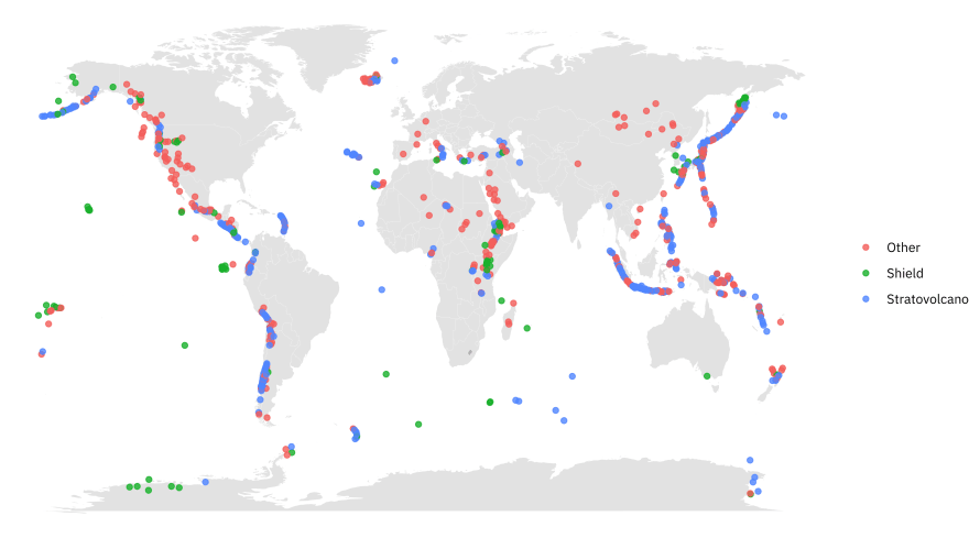
The biggest thing I know about volcanoes is the Ring of Fire 🔥 and there it is!

Build a model

Instead of splitting this small-ish dataset into training and testing data, let’s create a set of bootstrap resamples.

library(tidymodels)
volcano_boot <- bootstraps(volcano_df)

volcano_boot


## # Bootstrap sampling 
## # A tibble: 25 x 2
## splits id         
## <list> <chr>      
## 1 <split [958/350]> Bootstrap01
## 2 <split [958/340]> Bootstrap02
## 3 <split [958/353]> Bootstrap03
## 4 <split [958/354]> Bootstrap04
## 5 <split [958/359]> Bootstrap05
## 6 <split [958/350]> Bootstrap06
## 7 <split [958/356]> Bootstrap07
## 8 <split [958/353]> Bootstrap08
## 9 <split [958/354]> Bootstrap09
## 10 <split [958/360]> Bootstrap10
## # … with 15 more rows

Let’s train our multinomial classification model on these resamples, but keep in mind that the performance estimates are probably pessimistically biased.

Let’s preprocess our data next, using a recipe. Since there are significantly fewer shield volcanoes compared to the other groups, let’s use SMOTE upsampling (via the themis package) to balance the classes.

library(themis)

volcano_rec <- recipe(volcano_type ~ ., data = volcano_df) %>%
  update_role(volcano_number, new_role = "Id") %>%
  step_other(tectonic_settings) %>%
  step_other(major_rock_1) %>%
  step_dummy(tectonic_settings, major_rock_1) %>%
  step_zv(all_predictors()) %>%
  step_normalize(all_predictors()) %>%
  step_smote(volcano_type)

Let’s walk through the steps in this recipe.

• First, we must tell the recipe() what our model is going to be (using a formula here) and what data we are using.
• Next, we update the role for volcano number, since this is a variable we want to keep around for convenience as an identifier for rows but is not a predictor or outcome.
• There are a lot of different tectonic setting and rocks in this dataset, so let’s collapse some of the less frequently occurring levels into an "Other" category, for each predictor.
• Next, we can create indicator variables and remove variables with zero variance.
• Before oversampling, we center and scale (i.e. normalize) all the predictors.
• Finally, we implement SMOTE oversampling so that the volcano types are balanced!

volcano_prep <- prep(volcano_rec)
juice(volcano_prep)


## # A tibble: 1,383 x 14
## volcano_number latitude longitude elevation volcano_type tectonic_settin…
## <dbl> <dbl> <dbl> <dbl> <fct> <dbl>
## 1 213004 0.746 0.101 -0.131 Other -0.289
## 2 284141 0.172 1.11 -1.39 Other -0.289
## 3 282080 0.526 0.975 -0.535 Other -0.289
## 4 285070 0.899 1.10 -0.263 Other -0.289
## 5 320020 1.44 -1.45 0.250 Other -0.289
## 6 221060 -0.0377 0.155 -0.920 Other -0.289
## 7 273088 0.0739 0.888 0.330 Other -0.289
## 8 266020 -0.451 0.918 -0.0514 Other -0.289
## 9 233011 -0.873 0.233 -0.280 Other -0.289
## 10 257040 -0.989 1.32 -0.380 Other -0.289
## # … with 1,373 more rows, and 8 more variables:
## # tectonic_settings_Rift.zone...Oceanic.crust....15.km. <dbl>,
## # tectonic_settings_Subduction.zone...Continental.crust...25.km. <dbl>,
## # tectonic_settings_Subduction.zone...Oceanic.crust....15.km. <dbl>,
## # tectonic_settings_other <dbl>, major_rock_1_Basalt...Picro.Basalt <dbl>,
## # major_rock_1_Dacite <dbl>,
## # major_rock_1_Trachybasalt...Tephrite.Basanite <dbl>,
## # major_rock_1_other <dbl>

Before using prep() these steps have been defined but not actually run or implemented. The prep() function is where everything gets evaluated. You can use juice() to get the preprocessed data back out and check on your results.

Now it’s time to specify our model. I am using a workflow() in this example for convenience; these are objects that can help you manage modeling pipelines more easily, with pieces that fit together like Lego blocks. This workflow() contains both the recipe and the model, a random forest classifier. The ranger implementation for random forest can handle multinomial classification without any special handling.

rf_spec <- rand_forest(trees = 1000) %>%
  set_mode("classification") %>%
  set_engine("ranger")

volcano_wf <- workflow() %>%
  add_recipe(volcano_rec) %>%
  add_model(rf_spec)

volcano_wf


## ══ Workflow ════════════════════════════════════════════════════════════════════════
## Preprocessor: Recipe
## Model: rand_forest()
## 
## ── Preprocessor ────────────────────────────────────────────────────────────────────
## 6 Recipe Steps
## 
## ● step_other()
## ● step_other()
## ● step_dummy()
## ● step_zv()
## ● step_normalize()
## ● step_smote()
## 
## ── Model ───────────────────────────────────────────────────────────────────────────
## Random Forest Model Specification (classification)
## 
## Main Arguments:
## trees = 1000
## 
## Computational engine: ranger

Now we can fit our workflow to our resamples.

volcano_res <- fit_resamples(
  volcano_wf,
  resamples = volcano_boot,
  control = control_resamples(save_pred = TRUE)
)

Explore results

One of the biggest differences when working with multiclass problems is that your performance metrics are different. The yardstick package provides implementations for many multiclass metrics.

volcano_res %>%
  collect_metrics()


## # A tibble: 2 x 5
## .metric .estimator mean n std_err
## <chr> <chr> <dbl> <int> <dbl>
## 1 accuracy multiclass 0.661 25 0.00297
## 2 roc_auc hand_till 0.796 25 0.00304

We can create a confusion matrix to see how the different classes did.

volcano_res %>%
  collect_predictions() %>%
  conf_mat(volcano_type, .pred_class)


## Truth
## Prediction Other Shield Stratovolcano
## Other 2049 344 801
## Shield 223 585 204
## Stratovolcano 1251 179 3215

Even after using SMOTE oversampling, the stratovolcanoes are easiest to identify.

We computed accuracy and AUC during fit_resamples(), but we can always go back and compute other metrics we are interested in if we saved the predictions. We can even group_by() resample, if we like.

volcano_res %>%
  collect_predictions() %>%
  group_by(id) %>%
  ppv(volcano_type, .pred_class)


## # A tibble: 25 x 4
## id .metric .estimator .estimate
## <chr> <chr> <chr> <dbl>
## 1 Bootstrap01 ppv macro 0.643
## 2 Bootstrap02 ppv macro 0.659
## 3 Bootstrap03 ppv macro 0.656
## 4 Bootstrap04 ppv macro 0.639
## 5 Bootstrap05 ppv macro 0.580
## 6 Bootstrap06 ppv macro 0.651
## 7 Bootstrap07 ppv macro 0.680
## 8 Bootstrap08 ppv macro 0.617
## 9 Bootstrap09 ppv macro 0.636
## 10 Bootstrap10 ppv macro 0.651
## # … with 15 more rows

What can we learn about variable importance, using the vip package?

library(vip)

rf_spec %>%
  set_engine("ranger", importance = "permutation") %>%
  fit(
    volcano_type ~ .,
    data = juice(volcano_prep) %>%
      select(-volcano_number) %>%
      janitor::clean_names()
  ) %>%
  vip(geom = "point")

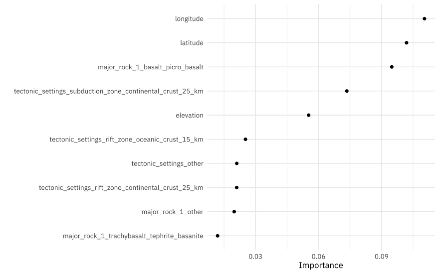
The spatial information is really important for the model, followed by the presence of basalt. Let’s explore the spatial information a bit further, and make a map showing how right or wrong our modeling is across the world. Let’s join the predictions back to the original data.

volcano_pred <- volcano_res %>%
  collect_predictions() %>%
  mutate(correct = volcano_type == .pred_class) %>%
  left_join(volcano_df %>%
    mutate(.row = row_number()))

volcano_pred


## # A tibble: 8,851 x 14
## id .pred_Other .pred_Shield .pred_Stratovol… .row .pred_class
## <chr> <dbl> <dbl> <dbl> <int> <fct>      
## 1 Boot… 0.474 0.149 0.377 1 Other      
## 2 Boot… 0.190 0.0771 0.733 3 Stratovolc…
## 3 Boot… 0.162 0.106 0.732 6 Stratovolc…
## 4 Boot… 0.233 0.0510 0.716 8 Stratovolc…
## 5 Boot… 0.206 0.0781 0.716 10 Stratovolc…
## 6 Boot… 0.351 0.0969 0.552 16 Stratovolc…
## 7 Boot… 0.428 0.0776 0.494 20 Stratovolc…
## 8 Boot… 0.148 0.0118 0.841 21 Stratovolc…
## 9 Boot… 0.258 0.389 0.352 26 Shield     
## 10 Boot… 0.433 0.457 0.110 29 Shield     
## # … with 8,841 more rows, and 8 more variables: volcano_type <fct>,
## # correct <lgl>, volcano_number <dbl>, latitude <dbl>, longitude <dbl>,
## # elevation <dbl>, tectonic_settings <fct>, major_rock_1 <fct>

Then, let’s make a map using stat_summary_hex(). Within each hexagon, let’s take the mean of correct to find what percentage of volcanoes were classified correctly, across all our bootstrap resamples.

ggplot() +
  geom_map(
    data = world, map = world,
    aes(long, lat, map_id = region),
    color = "white", fill = "gray90", size = 0.05, alpha = 0.5
  ) +
  stat_summary_hex(
    data = volcano_pred,
    aes(longitude, latitude, z = as.integer(correct)),
    fun = "mean",
    alpha = 0.7, bins = 50
  ) +
  scale_fill_gradient(high = "cyan3", labels = scales::percent) +
  theme_void(base_family = "IBMPlexSans") +
  labs(x = NULL, y = NULL, fill = "Percent classified\ncorrectly")